Building a Time Series Analysis Application

Key takeaways:

• Learn about the most common tasks in the journey of building a time series application
• Put theory into practice by building an example application in KNIME Analytics Platform

A complete time series analysis application covers the steps in a data science cycle from accessing to transforming, modeling, evaluating, and deploying time series data. However, for time series data the specific tasks in these steps differ in comparison to cross-sectional data.

For example: Cross sectional data are collected as a snapshot of one object at one point of time. Time series data are collected by observing the same object over a time period.

The regular patterns in time series data have their specific terminology, and they determine the required preprocessing before moving on to modeling time series.

Time series can be modeled with many types of models, but specific time series models, such as an ARIMA model, take use of the temporal structure between the observations.

Tutorial resources:

• The open source KNIME Analytics Platform, which you can download for free
• The workflow described in this article, which you can also download and use

Time series have various sources and applications: daily sales data for demand prediction, yearly macroeconomic data for long term political planning, sensor data from a smart watch for analyzing a workout session, and many more.

All these time series differ, for example, in their granularity, regularity, and cleanliness. For example:

• We can be sure that we have a GDP value for our country for this year, and for the next ten years, too, but we cannot guarantee that the sensor of our smart watch performs stably in any exercise and at any temperature.
• It could also be that time series data are not available at regular intervals, but can only be collected from random event points, such as disease infections or spontaneous customer visits.

What all these kinds of time series data have in common, though, is that they are collected from the same source over time.

Once we have the time series data, the next step is to make it equally spaced at a suitable granularity, continuous, and clean.

The required tasks depend on the original shape of the data and also our analytics purpose. For example, if we’re planning a one-week promotion of a product, we might be interested in more granular data than if we want to gain an overview of the sales of some product.

Time series need to be sorted by time. When you partition data into training and test sets remember to preserve the temporal structure between the records by taking data from top/bottom for testing/training.

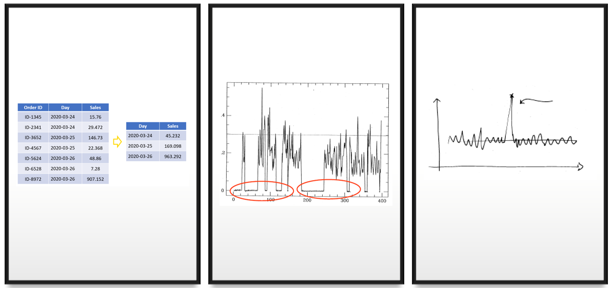
If your data contain more than one record per timestamp, then you need to aggregate them by the timestamp. For example, when you have multiple orders per day and you’re interested in the daily sales, you need to sum the sales for each day.

Furthermore, if you’re interested in the time series at another granularity than what you currently have in the data, for example, monthly sales instead of daily sales, you can further aggregate the data at the preferred granularity.

If some timestamps are missing, you need to introduce them to the time series in order to make it equally spaced. Sometimes the missing records are a part of the dynamics of the time series, for example, a stock market closes on a Friday and opens on a Monday.

When you introduce the missing timestamps to the data, the corresponding values are of course missing. You can impute these missing values by, for example, linear interpolation or moving average values. Remember, though, that the best technique for imputing missing values depends on the regular dynamics in the data.

For example:

• If you inspect weekly seasonality in daily data, and a value on one Saturday is missing, then the last Saturday’s value is probably the best replacement.
• If the missing values are not missing at random, like the missing stock market closing prices at weekends, you can replace them by a fixed value, which would be 0 in this case.
• If the missing values are random and they occur far enough in the past, you can use the data after the missing value, and ignore the older data.

One good way of handling rapid fluctuations and outliers is to smooth the data. Several techniques can be used, for example

• Moving average and exponential smoothing.
• Cutting the values that lie outside the whiskers of a box plot also smooths the data

Keep in mind that strong seasonality in the data might lead to a widespread box plot, and then it’s better to use a conditional box plot to detect outliers.

However, sometimes the time series is just showing a very irregular phenomenon! In such a case, you can try to make the time series more regular by extracting a subset of it, for example, by only considering the sales of one product instead of the sales of the whole supermarket, or by clustering the data.

At this point, we have our time series data in the shape that is suitable for exploring it visually and numerically. The different plots and statistics reveal long and short term patterns and temporal relationships in the time series that we can use to better comprehend the dynamics of it and predict its future development.

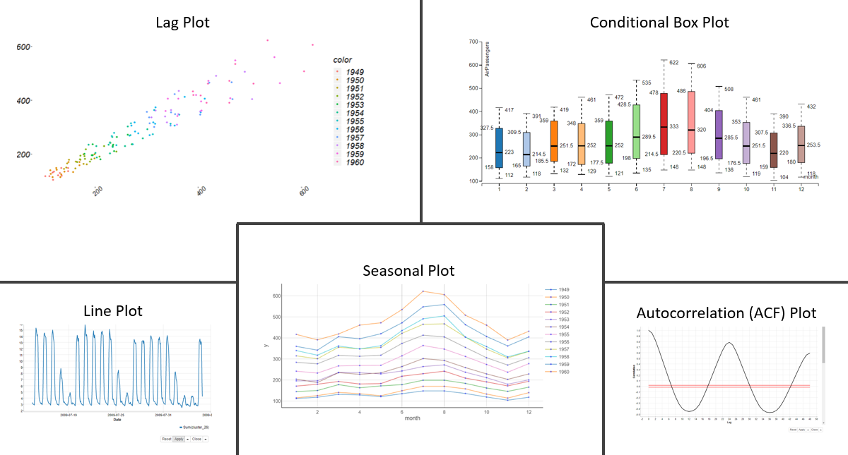
The basic plot for exploring time series is the line plot (see below) that shows a possible direction, regular and irregular fluctuations, outliers, gaps, or turning points in the time series.

If you observe a regular pattern in your time series, for example, yearly seasonality in the sales of beverages, you can then inspect each seasonal cycle (year) separately in a seasonal plot (below). In the seasonal plot you can easily see, for example, if July was a stronger sales month this year than last year, or if the monthly sales are increasing year by year.

If you’re interested in what happens within the seasons, for example, what is the median sales in the summer months and how much and to which direction the sales vary each month, you can inspect these kinds of dynamics in a conditional box plot (see below).

Yet another useful plot for exploring time series is the lag plot (see below). The lag plot shows the relationship between the current values and past values, for example, sales today and sales week before.

Classical decomposition, i.e. decomposing the time series into its trend, seasonalities, and residual provides a good benchmark for forecasting. The remaining part of the time series, the residual, is supposed to be stationary, and can be forecast by an ARIMA model, for example.

Remember, though, that if the residual series is not stationary, some additional transformations might be required, such as first order differencing, or log transformation of the original time series.

• Firstly, if the time series shows a direction, a trend, the time series can be detrended, for example, by fitting a regression model through the data, or by calculating a moving average value.

• Secondly, if the time series shows a regular fluctuation - a seasonality - the time series can be adjusted for it. You can find the lag where the major seasonality occurs in the autocorrelation plot of the time series.
  • For example, if you observe a peak at lag 7, and you have daily data, then the data will have weekly seasonality. The seasonality can be adjusted by differencing the data at the lag where the major spike occurs. If you want to adjust second seasonality in the data, you can do it by repeating the procedure for the adjusted (differenced) time series.

• Finally, when you have reached a stationary time series that is ready to be modeled by for example an ARIMA model, you can do a final check with, for example, Ljung-box test for stationarity.

Now we move on to modeling the residual part of the time series that contains its irregular dynamics. We can do this with:

• ARIMA models,
• Machine learning models
• Neural networks, and many variations of them

We often model the residual part of the time series by these models, because it’s stationary. However, decomposing the time series is not always necessary, because some models, like for example the seasonal ARIMA model, also work for modeling non-stationary time series.

In the following we collect a few properties of these different modeling techniques, their similarities and differences, so that you can pick the best one for your use case. Remember also that it’s useful to train multiple models, and even build an ensemble of them!

ARIMA (AutoRegressive Integrated Moving Average) model is a linear regression model between the current and past values (AR-part), and also between the current and past forecast errors (MA-part).

If the model has a non-zero I-part, then the data are differenced in order to make it stationary. Basic ARIMA models assume that the time series is stationary, and stationary time series don’t have predictable patterns in the long term.

The declining accuracy in the long term forecasts can be seen in the increasing confidence intervals of the forecasts.

Having more data is not always better for training ARIMA models: Large datasets might make estimating the model parameters of an ARIMA model time consuming, as well as exaggerate the difference between the true process and the model process.

Machine learning models use the lagged values as predictor columns, and they ignore the temporal structure between the target column and predictor columns.

Machine learning models can also identify long term patterns and turning points in the data, provided that enough data are provided in the training data to establish these patterns. In general, the more irregularities the data shows, the more data are needed for training the model.

When you apply a machine learning model, it’s recommended to model the residual. Otherwise, you might build a model that’s more complicated than the classical decomposition model, but which is actually not learning anything new on top of that!

1. Some phenomena are difficult to forecast, and in such a case it often makes sense to go for a simpler model and not invest resources in modeling something that cannot be forecast accurately.
2. The model’s performance is not the only criterion. If important decisions are based on the results of the model, it’s interpretability might be more important than a slightly better performance. That said, a neural network might lose against a simple classical decomposition model although it forecast slightly better.
3. Adding explicative variables to your model might improve the forecast accuracy. However, in such a model the explicative variables need to be forecast, too, and the increasing complexity of the model is not always worth the better accuracy. Sometimes rough estimates are enough to support the decisions: if shipping amounts are calculated in tens and hundreds, then the forecast demand doesn’t have to have a greater granularity either.

After training a model, the next step is to evaluate it. For in-sample forecasting, the test set is the training set itself, so the model process is fitted to the data that were used for training the model. For out-of-sample forecasting, the test set is subsequent to the training set in time.

One recommended error metric for evaluating a time series model is the mean absolute percentage error (MAPE), since it provides the error in a universal scale, as a percentage of the actual value. However, if the true value is zero, this metric is not defined, and then also other error metrics, like the root mean squared error (RMSE), will do.

What is often recommended, though, is to NOT to use R-squared. The R-squared metric doesn’t fit the context of time series analysis because the focus is on predicting future systematic variability of the target column instead of modeling all variability in the past.

We’re almost there! The last step is to forecast future values and reconstruct the signal.

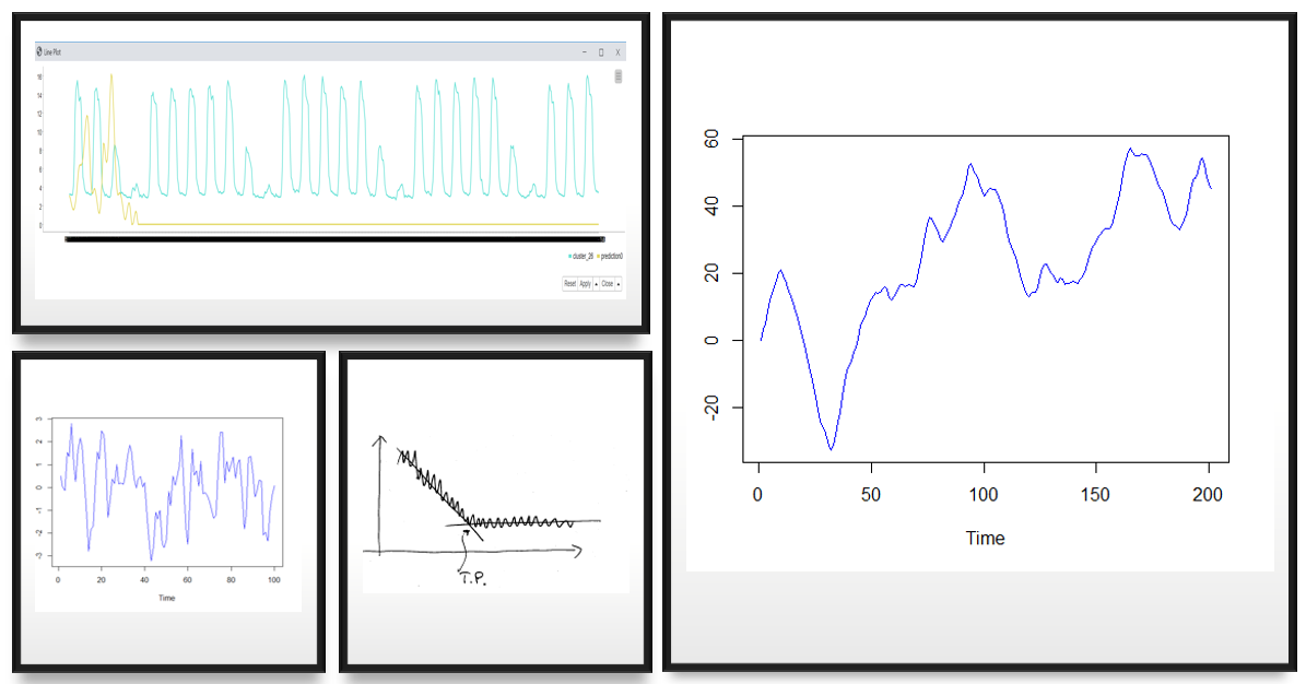
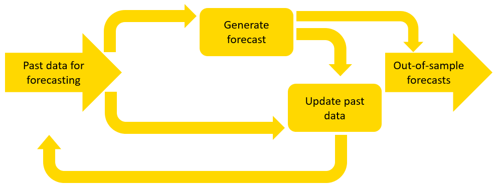
If you have a model that cannot provide accurate forecasts in the long term, dynamic deployment often improves the out-of-sample forecast accuracy.

In dynamic deployment, only one point in the future is forecast at a time, and the past data are updated by this forecast value to generate the next forecast (see below).

Finally, if we decompose the time series before forecasting, we need to restore the trend and/or seasonalities to the forecasts.

If we adjust the seasonality by differencing the data, we start reconstructing the signal by adding values at the lag where the seasonality occurs.

For example, if we had daily data y where we applied seasonal differencing at lag 7 (weekly seasonality), restoring this seasonality would require the following calculation to the forecast values y_t+1, y_t+2, ..., y_t+h:

where ti s the last time point in the training data, and h is the forecast horizon.

In order to restore second seasonality, we would repeat the step described above for the restored time series.

If we wanted to restore the trend component to the time series, we would apply the regression model representing the trend to the restored time series.

Now, let’s take a look at how to turn these steps into practice using KNIME Analytics Platform.

KNIME Analytics Platform is free and open-source software that you can download to access, blend, analyze, and visualize your data, without any coding. Its low-code, no-code interface makes analytics accessible to anyone and provides an advanced data science set of tools for experienced users.

The workflow Accessing Transforming and Modeling Time Series (available on the KNIME Hub).

Below, you can see the steps from accessing to cleaning, visually exploring, decomposing and modeling time series.

For some of these tasks, we use time series components that encapsulate workflows as functionalities specific to time series: aggregate the data at the selected granularity, perform the classic decomposition, and more.

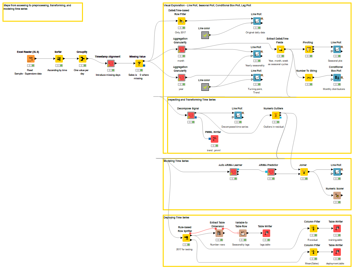
In this example, we use the Sample - Superstore data provided by Tableau. In our analysis we focus on the orders of all products from 2014 to 2017, altogether 9994 records.

• We start the preprocessing by reshaping the data into time series data by calculating the total sales per day.
• Now, we only have one value per day, but some days are missing because no orders were submitted on these days.
• Therefore, we introduce these days to the time series and replace the missing sales values with a fixed value 0.
• After that, we aggregate the data at the monthly level, and consider the average sales in each month in further analysis.

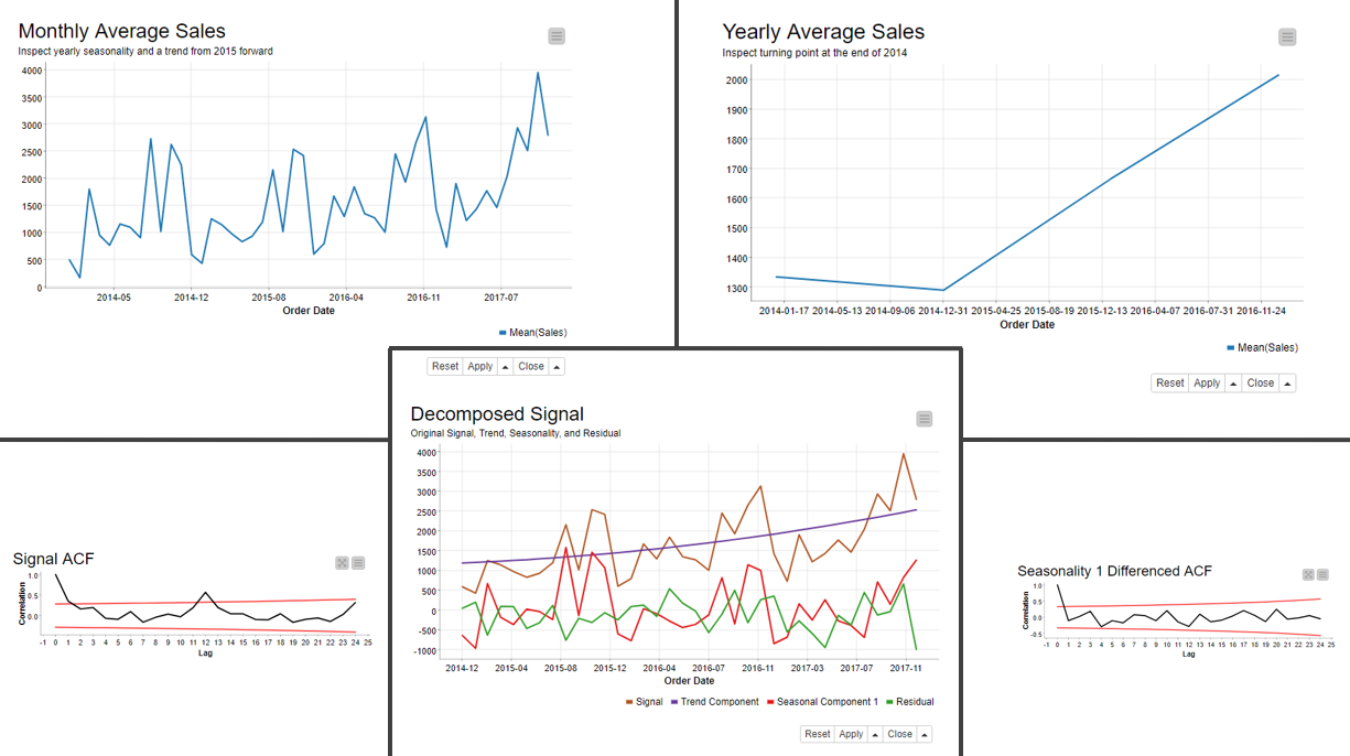
For visual exploration, we also aggregate the data at a yearly level, and we find out that there’s a turning point at the beginning of the year 2015, as the line plot on the right, as shown below.

The line plot on the left shows the yearly seasonality in the data: there are two regular peaks at the end of each year, and a lower peak at the beginning of each year.

We also detect yearly seasonality in the data, as shown by the major spike at the lag 12 in the ACF plot on the left.

We decompose the time series into its trend, seasonality, and residual, and these components are shown in the line plot in the middle of the screenshot shown below.

The ACF plot on the right shows no significant autocorrelation in the residual series.

Next, we model the residual series of the monthly average sales with an ARIMA model.

After differencing at the lag 12, the length of the time series is 36 observations. We look for the best model with the Auto ARIMA Learner component with max order 4 for the AR and MA parts and max order 1 for the I part.

The best performing model based on Akaike information criterion is ARIMA (0, 1, 4), and the resulting MAPE based on in-sample forecasts is 1.153.

Finally, we assess the model’s out-of-sample forecast accuracy. The workflow Forecasting and Reconstructing Time Series (available on the KNIME Hub), which you can see below, shows how to forecast the daily sales in 2017 based on the monthly data in the years 2014 to 2016 (24 observations), and the winning ARIMA (0,1,4) model using the dynamic deployment approach.

After that, we reconstruct the signal, in this case, restore the trend and yearly seasonality to the forecast values (12 monthly average sales values). We compare the actual and forecast values, and obtain an MAPE of 0.336.

Time series, be it sensor data showing the behavior of a tiny object nanosecond after nanosecond, macroeconomic data for the 20th century, or something in-between, have specific analytics techniques that apply to accessing, manipulating, and modeling steps.

In this article, we have introduced you to the basics of analytics techniques for time series that help you to get started when you’re working with time series data.

• [1] Chambers, John C., Satinder K. Mullick, and Donald D. Smith. How to choose the right forecasting technique. Harvard University, Graduate School of Business Administration, 1971.
• [2] Hyndman, Rob J., and George Athanasopoulos. Forecasting: principles and practice. OTexts, 2018.