Know Your Chances: Calculate Probability in KNIME

How likely are you to get wet in the rain this evening or win a multi-million dollar lottery or even become the next president of the US? These questions can all be answered using probability. For example, weather forecasters assess how likely it is that there will be rain, snow etc. on a given day in a certain area using probability. So when your local forecasters tell you “there is an 85% chance of rain today between 5PM and 8PM” to indicate that it is likely to rain during certain hours, it’s wise for you to stay indoors.

Probability is used in many situations such as sports betting where companies determine the odds they should set for certain teams to win certain games or by health insurance companies when they determine how likely it is that certain individuals spend a certain amount on healthcare each year.

Even Doctor Strange used probability to determine that there was only one in 14 million possibilities for the Avengers to win against Thanos.

To understand the importance of probability, in this article we want to use KNIME Analytics Platform to extract insights from the Adult.csv dataset by calculating different probabilities.

Key Takeaways:

Get a theoretical background of what probability is

Get an overview of different formulas for calculating probabilities

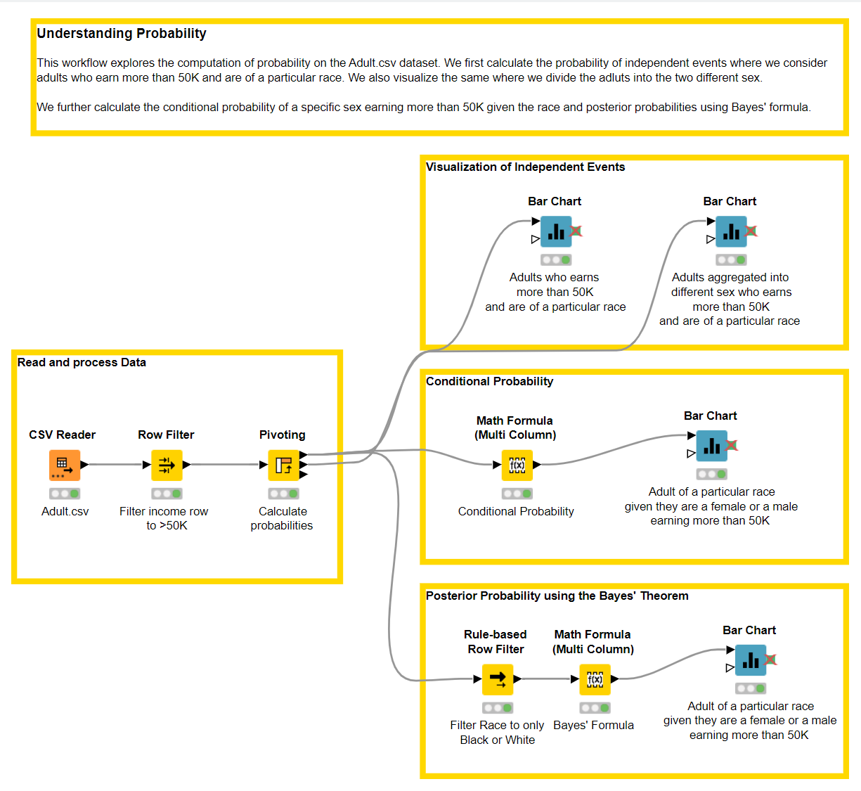
Learn to build a workflow to calculate probabilities using KNIME Analytics Platform

Download our Probabilities workflow for free from the KNIME Hub

The game of cricket starts with a toss, i.e. flipping a coin to determine which captain will have the right to choose whether their team will bat or field at the start of the match. If we assume a fair coin, each captain’s team has an equal chance to bat or field. Probability helps us answer questions regarding how likely or unlikely it is for an event to occur. We know that heads is just as likely to show up as tails. The probability of an event to occur is a value that tells us how likely that event is to happen.

There are two possible outcomes when tossing a coin: heads and tails. The probability of the coin landing on either side is 50%. Let’s see how this is calculated:

On tossing a coin, the probability of heads is:

P(Head) = P(H) = ½

And similarly, the probability of tails is:

P(Tails) = P(T) = ½

To understand what this value means, let’s look into the Probability number line:

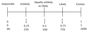
When the probability of an event is 0 it means that the event cannot happen, i.e. impossible. For example, the probability of the earth being flat is zero. When the probability of an event is 1 it means that the event is definitely going to happen, i.e. certain. For example, the probability of tomorrow being Thursday if today is Wednesday is 1. Events cannot be less likely than impossible and more likely than certain, and if there is a chance that an event will happen, then its probability is between zero and one.

If the probability of an event is ½, like in our coin toss example, it means that an event is just as likely to happen as it is to not happen. When the probability of the event is less than ½ the event is said to be unlikely to occur, and similarly, if it is more than ½ then it is said to be likely to occur.

In the following section, we will look into the relationship between two events and how the calculation of probability can change if the events are mutually exclusive, that is two events cannot happen at the same time, and if the events are non-mutually exclusive, that is the events can happen at the same time.

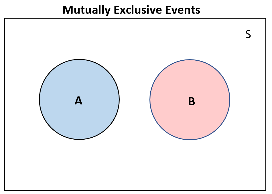
Mutually exclusive events occur when two events cannot happen at the same time or simultaneously. They are also called disjoint events. An easy example is winning or losing a game. These two events are disjoint since you can either win the game or lose the game and they cannot happen at the same time. When two events (call them "A" and "B") are mutually exclusive the probability of A and B to occur together equals 0 (impossible). Below we have a Venn diagram of the mutually exclusive events which shows the same.

However, for mutually exclusive events, we can compute the probability of A or B to occur by summing their individual probabilities. For example, let’s take a fair die and calculate the probability of rolling a 6 or less than or equal to a 2:

P(A∪B) = P(A) + P(B)

The probability of rolling a 6 is P(A) = 1/6, and the probability of rolling a 1 or a 2 is P(B) = 2/6. Hence, we calculate the probability as:

P(6 or ≤ 2) = 1/6 + 2/6 = 1/2

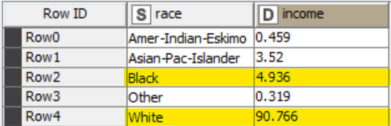
Let’s look into a more articulated example where we use KNIME Analytics Platform. The dataset that we consider is the Adult.csv, and we are interested in the columns race, sex and income where individuals earn more than 50K.

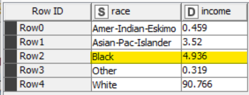
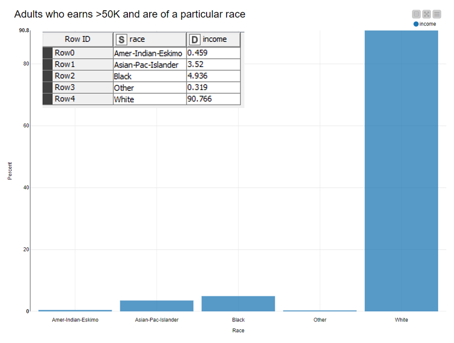
The table below shows the probability of adults earning more than 50K expressed in percentage (income column) and their specific race. To understand mutually exclusive probability, we can see that the rows displayed in the table are disjoint from each other. That is, a white adult earning more than 50K cannot simultaneously be a black adult earning more than 50K.

If we were to apply the same formula above for calculating mutually exclusive events, we would obtain:

P(Black adult earning > 50K or White adult earning > 50K) =

P(Black adult earning > 50K) + P(White adult earning > 50K)

Using the values (in percentage) highlighted in the table above we can say that:

P(Black adult earning > 50K or White adult earning > 50K) = 4.936 + 90.766 = 95.702

Using this dataset, the probability of an adult being black or of white and earning more than 50K is 0.957.

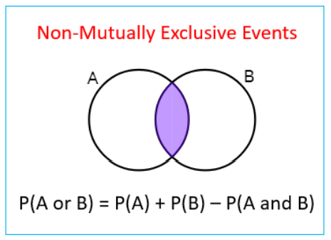
Non-mutually exclusive events are events that can happen at the same time, i.e. simultaneously. For example, having a cold and a headache at the same time.

Let’s consider non-mutually exclusive events with an example. Suppose we have a standard deck containing 52 French-suited playing cards. Let’s first calculate the probability of drawing a Queen or Hearts.

Since the two events can occur at the same time, we can compute the probability as:

P(A∪B) = P(A) + P(B) - P(A∩B)

The probability of picking a Queen from the deck is P(A) = 4/52, since there are 4 queens of different suits. Next, the probability of picking a Heart is P(B) = 13/52. The probability of picking a card that is both a Queen and a Heart P(A∩B)=1/52 since there can only be one queen of hearts. Hence, we compute the probability of non-mutually exclusive events to be:

P(Queen or Hearts) = P(Queen) + P(Heart) - P(Queen and Heart) = 4/52 + 13/52 - 1/52 = 4/13

Going back to our example using the Adult dataset, let’s calculate the probability of an adult being black or of an adult being male and earning more than 50K. Since both events can happen at the same time and are not mutually exclusive, we will use the above formula:

P(Black adult or Male adult earning > 50K) = P(Black adult) + P(Male earning > 50K) - P(Black adult and Male adult earning > 50K)

Using the Pivoting node, we obtain the “Group totals” table displayed below:

Through the groups table, we obtain the probability of an adult being black:

P(A) = P(Black adult) = 4.936

The “Pivot totals” table displayed below returns the probability of an adult being male and earning more than 50K.

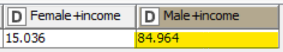
P(B) = P(Male adult earning > 50K) = 84.964

From the “Pivot table”, we get the probability of an adult being black and male earning more than 50K.

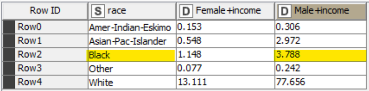
P(A∩B) = P(Black adult and Male adult earning > 50K) = 3.788

Hence, we obtain in percentage:

P(Black adult or Male adult earning > 50K) = P(Black adult) + P(Male earning > 50K) - P(Black adult and Male adult earning > 50K)

P(A∪B) = 4.936 + 84.964 - 3.788 = 86.112

That is the probability of these two non-mutually exclusive events is 0.861.

In the example above, we calculated the probability of mutually exclusive and non-mutually exclusive events. Independent events are events whose occurrence does not depend on any other events. That is, we can roll a die and also pick a card from a deck independently, since the occurrence of one event will not affect the other. This is also known as joint probability.

Now to understand independent events from our theoretical example, let’s find the probability of rolling a die ≤ 2 and drawing a card which is of the suits Hearts. These two events are said to be independent since the probability of picking a particular card is completely independent of rolling a number on a die. The formula to calculate joint probability is :

P(A∩B) = P(A) * P(B)

From the formula above, we can derive that the probability of rolling a die ≤ 2 is P(A) = 2/6, and similarly the probability of drawing a card which is of Hearts is P(B) = 13/52. Hence we obtain:

P(Die ≤ 2 and card being Hearts) = 2/6 * 13/52 = 1/12

In our practice dataset, adults belonging to a certain race and sex, and earning more than 50K are dependent events, i.e. the occurrence of one event effects the occurrence of the other event. Therefore, we need to introduce and understand the concept of conditional probability

Conditional probability measures the probability of an event to occur given that another event has already occurred. Let’s consider two events, event A and event B. Given the outcome of event B, we are interested in the probability of event A. Since the two events are dependent on each other, the knowledge of the occurrence of event B will impact the occurrence of event A. Conditional probability is calculated using the following formula:

P(A|B) = P(A ∩ B)P(B)

Conditional probability of A given B i.e. the probability of event A occurring given that event B has already occurred, is equivalent to the joint probability of events A and B divided by the probability of event B.

Let’s see a simple example. For a standard 52-card deck, given that you drew a black card, what is the probability that it is a ten?

P(10 | Black card) = P(10 and Black card) / P(Black card)

Out of all the black cards, there are two tens, the ten of spades and the ten of clubs. Hence, we have:

P(10 | Black) = (4/52 * 26/52) / 26/52 = 1/13

So far we looked into calculating specific probability values such as in our card example but how do we calculate conditional probability of the data if we have new information or prior knowledge about how likely events are to occur? To tackle such situations, we can use Bayes’ theorem. It provides a way to incorporate new information about an event in the computation of probability. In other words, it provides a way to revise the existing predictions, i.e. update the probability when given new or additional information. For example, it is often used in the financial sector to calculate and update risk. In machine learning, Bayes’ theorem is applied by a number of models, such as the naive Bayes classifiers.

This theorem relies on incorporating prior probability in order to compute posterior probability. Prior probability refers to the probability of the event occurring before the new information or data has been collected. That is, the probability is calculated using the current knowledge. Posterior probability refers to the revised or the updated probability that is calculated by taking into account the new information in order to produce more accurate results from the data. The formula for calculating Bayes’ theorem is:

P(A|B) = P(A ∩ B)P(B) = P(A) * P(B|A)P(B)

From the above formula we apply Bayes’ theorem to event A given B, i.e., the probability of event A occurring given that event B has already occurred. The latter is equivalent to the probability of event A multiplied by the conditional probability of B given A, and divided by the probability of event B.

Let’s now calculate conditional probability using KNIME Analytics Platform on the Adult.csv dataset. Similar to our previous examples, we will look into the columns race and sex for adults whose income is more than 50K.

We first calculate the joint probability using the Pivoting node, where we look at adults who earn more than 50K and belong to a particular race (Fig. 5).

We use the joint probability formula which is given by:

P(A∩B) = P(A) * P(B)

P(adults earning >50K and White) = P(Adults earning >50K) * P(White) = 90.766

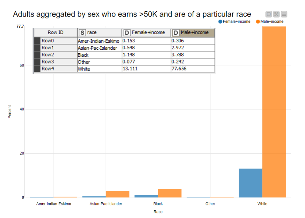
We can further split the same graph into males and females who earn more than 50K and are of a particular race (Fig. 6). We use the same formula as above to calculate this probability:

P(A∩B) = P(A) * P(B)

P(Female earning >50K and White) = P(Female earning >50K) * P(White) = 13.111

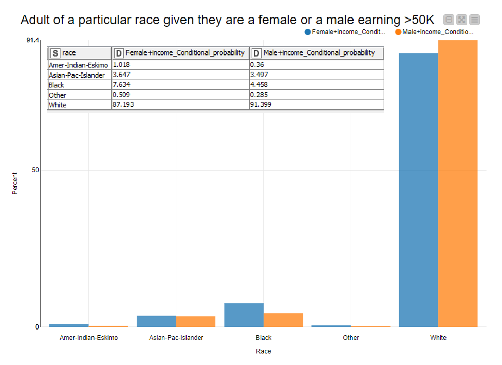
Now, we can calculate conditional probability. In this case, we look at the probability of an adult to belong to a particular race given they are a female or a male earning more than 50K.

The formula we use to calculate conditional probability is:

P(A|B) = P(A ∩ B)P(B)

For example, let’s calculate in percentage the probability of a black adult given she is a female earning more than 50K. For this, we have the formula:

P(Black adult | Female earning >50K) = P(Black adult ∩ Female earning >50K) / P(Female earning >50K)

In Fig. 7, we can see that the probability of an adult being black given that she is a female earning more than 50K is 7.634 (in percent).

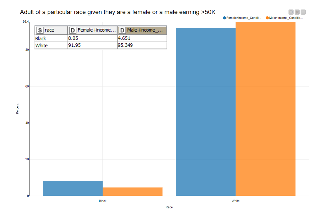
From the above, calculating conditional probability helps us to see how the two events relate to one another. But what if we have new information, such as more number of races to account for or we take in account only two races to calculate probabilities? In such cases, we use Bayes’ theorem. We can now use the values above as the prior probabilities i.e. calculating the probability before having the knowledge of the new information, and we update the same with new information to calculate posterior probabilities

Let’s take only two races in account, black and white, and consider this to be the new information for calculating posterior probability using Bayes’ theorem. We update our data and calculate probabilities for an adult of race black or white given gender and earnings >50K using Bayes’ theorem. We can do so using the formula we have:

P(A|B) = P(A) * P(B|A)P(B)

To calculate the posterior probability after incorporating our new information we have:

P(Black adult | Female earning > 50K) = P(Black adult) * P(Female earning >50K | Black adult) / P(Female earning >50K)

In Fig. 8, we can see that the probability of an adult being black given that she is a female earning more than 50K is 8.05 (in percent).

We see the difference between the prior probability and the posterior probability after integrating new pieces of information into our data.

When we study probability, we often take simple examples, be it a coin toss or a die roll. In those cases, computing probabilities is straightforward and your pen and copybook would suffice. However, when we work with real datasets and we need to compute and understand different probabilities for categories of our data, we need a more sophisticated approach.

In this blog post, we explored different theoretical concepts parallelly with examples built in KNIME Analytics Platform. We used the Adult.csv dataset to show how to calculate a single probability, joint probability, conditional probability, and Bayes’ theorem.

Using KNIME Analytics Platform and its Pivoting and Math Formula nodes, we can perform step-by-step computations and find probabilities in an easy and codeless fashion. Additionally, we can use the Bar Chart node to visualize and inspect our results.