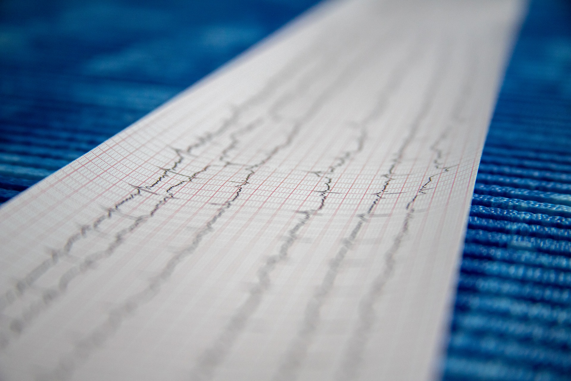
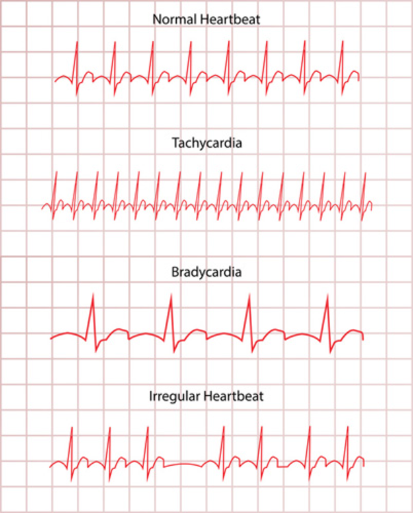
How to perform ECG categorization and detect arrhythmia

Arrhythmia is a varying rhythm in one’s heartbeat. It happens when signals from the brain to the heart are not able to regulate its beat normally. As a result, the heart will beat too quickly (tachycardia) or slowly (bradycardia). (Fig. 1).

This blog continues our look at ECG classification with deep learning, using the ECG heartbeat categorization dataset on Kaggle. In this article I want to discuss how to tackle multiclass classification: The dataset, which was compiled and pre-processed from PhysioNet’s MIT-BIH Arrhythmia Database, contains five different types of beat categories.

Fig. 1: Differentiation between kinds of arrhythmia.

PhysioNet's MIT-BIH Arrhythmia Data

The ECG heartbeat categorization dataset on Kaggle is composed of two collections of heartbeat signals taken from two famous datasets in heartbeat classification, the MIT-BIH Arrhythmia dataset and the PTB diagnostic ECG database. In our first article about ECG classification with deep learning, we trained our model on the PTB dataset, which has 2 categories of heartbeat signals. In this article, we are going to be training our model on the MIT-BIH Arrhythmia dataset, which contains 5 different heartbeat signal categories.

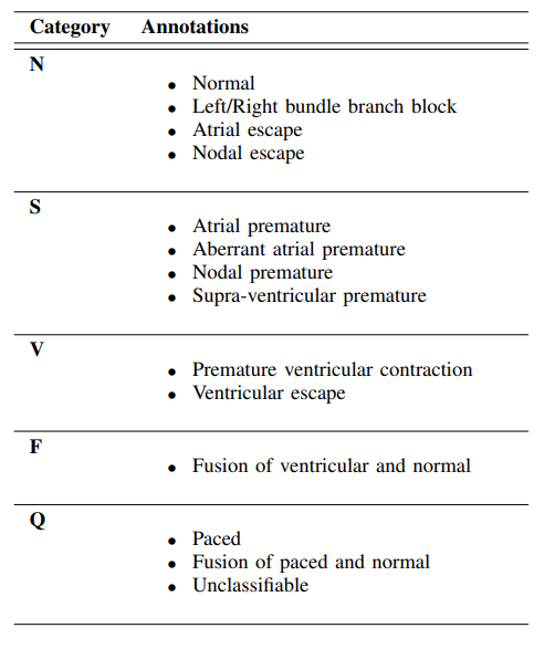
In the Kaggle heartbeat dataset you'll find “mitbih_train.csv” and “mitbih_test.csv.” among the four files. As the names suggest, we have one file for model training purposes and another for testing purposes. There are 188 columns in each file, just like for the PTB dataset. The target column has five class attributes: 0,1,2,3, and 4. These are their definitions:

0 - “N” for normal heartbeats
1 - “S” for supra-ventricular premature
2 - “V” for ventricular escape
3 - “F” for fusion of ventricular and normal
4 - “Q” for unclassified heartbeats

Details for each of the classes can be found in Fig. 2, with the descriptions from the associated research paper by the authors.

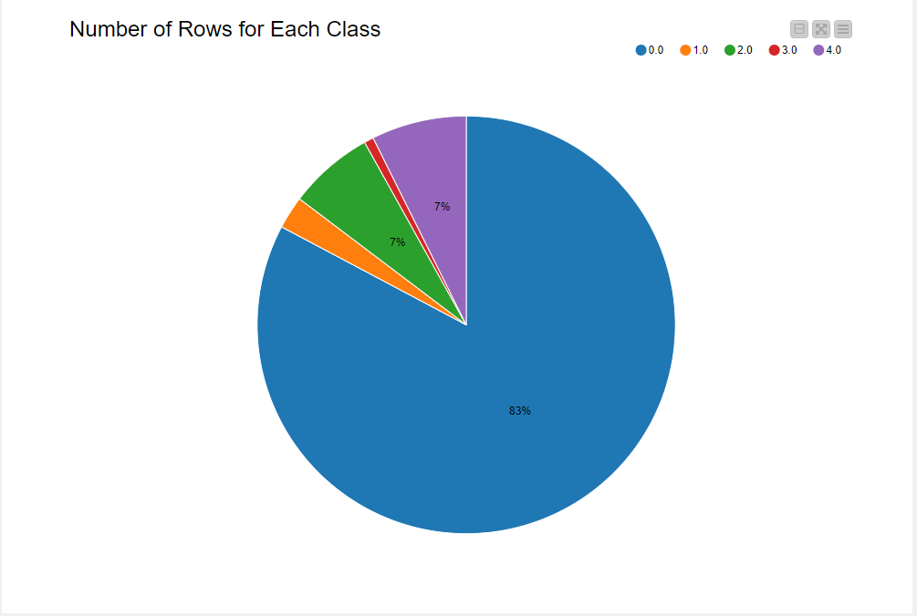
Fig.2: Detailed description of all class variables in the MIT-BIH arrhythmia dataset.

The training set has 87,554 rows, while the test set has 21,892 rows. The train set is highly imbalanced, with normal heartbeats labeled “0.0” (83% from Fig. 3). Next I’ll discuss my data preparation approach to train an unbiased model.

Fig. 3: Class distribution in training set. Imbalance is evident here.

Treating class imbalance for multiple classes

For an unbiased model, class variables were shuffled and converted to string. I visualized the distribution of rows in the training set (the blue annotation block in Fig. 4). Class variables are one-hot encoded and splitted such that the bottom port outputs all rows corresponding to “normal” class and rest in the top port. Using the “Bootstrap Sampling” node, the “normal” class is downsampled to return 25% of total normal heartbeats in the dataset. The downsampled table is concatenated with the rest of the rows belonging to other classes. The resulting table is manipulated using a “SMOTE” node by oversampling minority classes.

Using SMOTE on a large dataset with multiple class variables is a time-consuming process. To make it relatively faster, downsampling of the majority class is carried out before oversampling. The final output now has equal proportions of rows. “CSV Writer'' is used to write the updated table in the data area of the workflow to avoid repeating the process and save time (Fig. 4).

Fig.4: Downsampling the majority class and using SMOTE to oversample the minority classes.

Model Training

Now that my data is resampled, I will proceed with the data modeling. Training data is partitioned with 80/20 split. Since test data is already provided, 20% of partitioned data was used for validation on each epoch by Keras Network Learner Node.

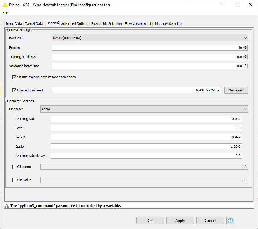
The neural network used is the same as in Part 1 of the blog. However, since it's a multiclass problem, the loss function used here is “Categorical Cross-Entropy,” and it’s optimized using Adam in Keras Network Learner Node. The rest of the optimizer settings can be seen in Fig. 5. Training the model took around 5 minutes and 37 seconds, with a validation accuracy of approximately 97%.

Fig.5: Configuration window of Keras Network Learner Node.

Model Scoring

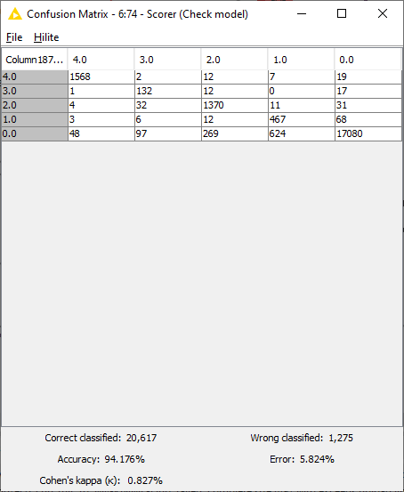
Similarly to the workflow from Part 1, a Keras Network Executor Node is used to make predictions on the test set provided by the authors. The “Many to One” node is used to extract predictions with maximum probability, while model performance is measured using the “Scorer“ node. As seen in Fig. 6, the model makes predictions with 94.1% accuracy, with 20,617 rows correctly identified and 1,275 wrongly classified.

Fig. 6: Confusion Matrix of Model performance

Conclusion

In this second article on ECG classification, I have discussed an arrhythmia dataset, which is available on Kaggle. The dataset was highly imbalanced, with the majority class being “Normal Heartbeat.” The imbalance was adjusted using Bootstrap Sampling (downsampling) of the majority class and oversampling of the minority class using the SMOTE technique.

Similarly to before, data was trained using 1-Dimensional Convolutional Neural Network architecture, including Batch Normalization and Max Pooling. The model performed with a higher accuracy on the test set. The complete workflow can be found on the KNIME Hub under the Digital Health public space.

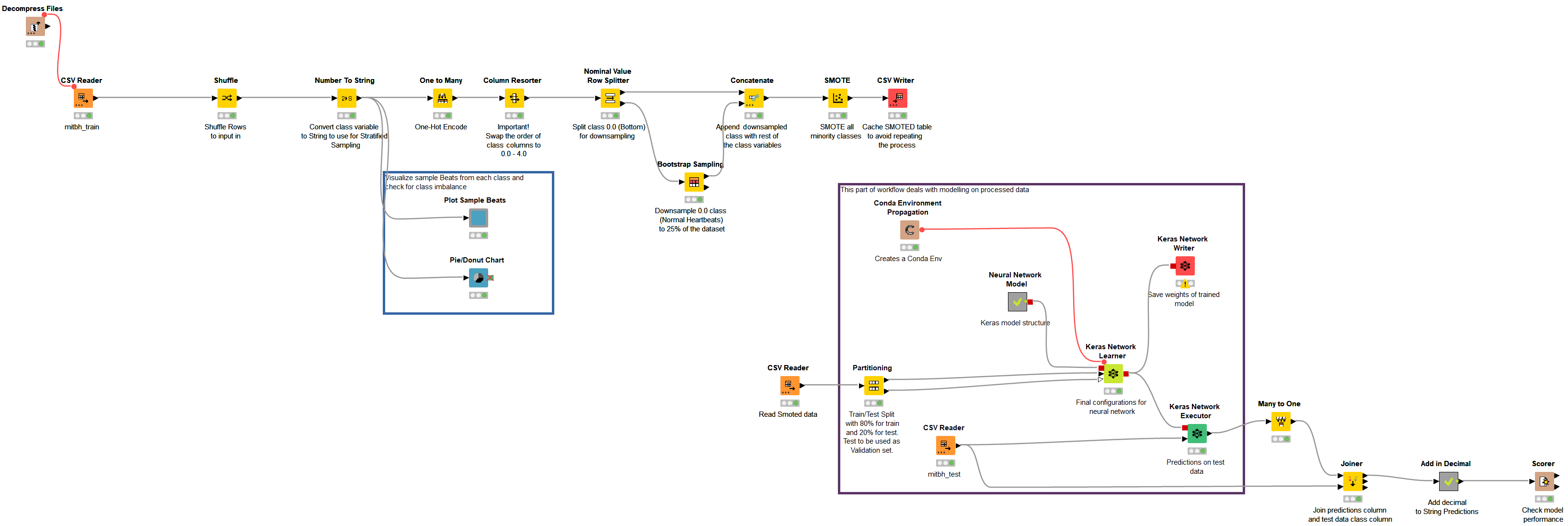
Fig. 7: Complete workflow of ECG arrhythmia classification in KNIME.

The workflow group comprising the ECG arrhythmia classification on the KNIME Hub is ECG PTB and MIT-BIH Data Analysis & Modeling,” under the name “ecg_cnn_mit.” Figure 7 shows the main workflow of the ECG classification using the arrhythmia dataset.