Let’s Talk Confusion Matrix and Class Statistics

Wheeling like a hamster in the data science cycle? Don’t know when to stop training your model? Model evaluation is an important part of a data science project and it’s exactly this part that quantifies how good your model is, how much it has improved from the previous version, how much better it is than your colleague’s model, and how much room for improvement there still is. In this series of blog posts, we review different scoring metrics: for classification, numeric prediction, unbalanced datasets, and other similar more or less challenging model evaluation problems.

This first blog post lauds the confusion matrix - a compact representation of the model performance, and the source of many scoring metrics for classification models.

A classification model assigns data to two or more classes. Sometimes, detecting one or the other class is equally important and bears no additional cost. For example, we might want to distinguish equally between white and red wine. At other times, detecting members of one class is more important than detecting members of the other class: an extra investigation of a non-threatening flight passenger is tolerable as long as all criminal flight passengers are found.

Class distribution is also important when you’re quantifying performances of classification models. In disease detection, for example, the number of disease carriers can be minor in comparison with the class of healthy people.

The first step in evaluating a classification model of any nature is to check its confusion matrix. Indeed, a number of model statistics and accuracy measures are built on top of this confusion matrix.

Let’s take the case of the email classification problem. The goal is to classify incoming emails in two classes: spam vs. useful (“normal”) email. For that, we use the Spambase Data Set provided by UCI Machine Learning Repository. This dataset contains 4601 emails described through 57 features, such as text length and presence of specific words like “buy”, “subscribe”, and “win”. The “Spam” column provides two possible labels for the emails: “spam” and “normal”.

Figure 1 shows a workflow that covers the steps to build a classification model: reading and preprocessing the data, partitioning into a training set and a test set, training the model, making predictions by the model, and evaluating the prediction results.

• Download the Evaluating Classification Model Performance workflowfrom the KNIME Hub.

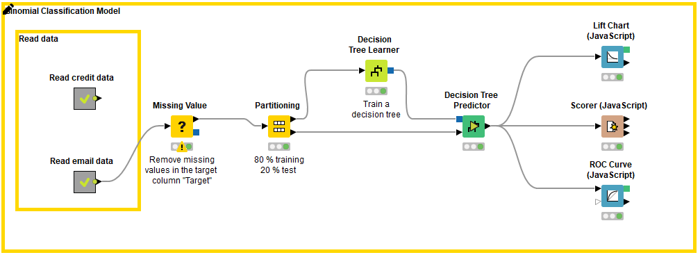
The last step in building a classification model is model scoring, which is based on comparing the actual and predicted target column values in the test set. The whole scoring process of a model consists of a match count: how many data rows have been correctly classified and how many data rows have been incorrectly classified by the model. These counts are summarized in the confusion matrix.

In the email classification example we need to answer several different questions:

• How many of the actual spam emails were predicted as spam?
• How many as normal?
• Were some normal emails predicted as spam?
• How many normal emails were predicted correctly?

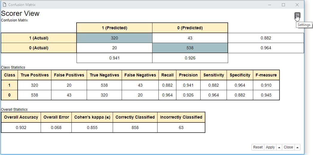
These numbers are shown in the confusion matrix. And the class statistics are calculated on top of the confusion matrix. The confusion matrix and class statistics are displayed in the interactive view of the Scorer (JavaScript) node as shown in Figure 2.

Let’s see now what these numbers are in a confusion matrix.

The confusion matrix was initially introduced to evaluate results from binomial classification. Thus, the first thing to do is to take one of the two classes as the class of interest, i.e. the positive class. In the target column, we need to choose (arbitrarily) one value as the positive class. The other value is then automatically considered the negative class. This assignment is arbitrary, just keep in mind that some class statistics will show different values depending on the selected positive class. Here we chose the spam emails as the positive class and the normal emails as the negative class.

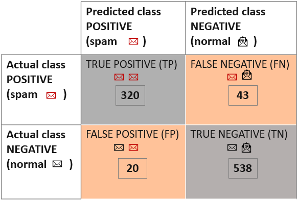
The confusion matrix in Figure 3 reports the count of:

• The data rows (emails) belonging to the positive class (spam) and correctly classified as such. These are called True Positives (TP). The number of true positives is placed in the top left cell of the confusion matrix.

• The data rows (emails) belonging to the positive class (spam) and incorrectly classified as negative (normal emails). These are called False Negatives (FN). The number of false negatives is placed in the top right cell of the confusion matrix.

• The data rows (emails) belonging to the negative class (normal) and incorrectly classified as positive (spam emails). These are called False Positives (FP). The number of false positives is placed in the lower left cell of the confusion matrix.

The data rows (emails) belonging to the negative class (normal) and correctly classified as such. These are called True Negatives (TN). The number of true negatives is placed in the lower right cell of the confusion matrix.

Therefore, the correct predictions are on the diagonal with a gray background; the incorrect predictions are on the diagonal with a red background:

Now, using the four counts in the confusion matrix, we can calculate a few class statistics measures to quantify the model performance.

The class statistics, as the name implies, summarizes the model performance for the positive and negative classes separately. This is the reason why its value and interpretation changes with a different definition of the positive class and why it is often expressed using two measures.

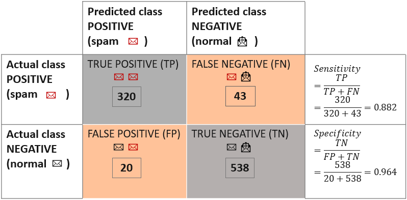
Sensitivity measures how apt the model is to detecting events in the positive class. So, given that spam emails are the positive class, sensitivity quantifies how many of the actual spam emails are correctly predicted as spam.

We divide the number of true positives by the number of all positive events in the dataset: the positive class events predicted correctly (TP) and the positive class events predicted incorrectly (FN). The model in this example reaches the sensitivity value of 0.882. This means that about 88 % of the spam emails in the dataset were correctly predicted as spam.

Specificity measures how exact the assignment to the positive class is, in this case, a spam label assigned to an email.

We divide the number of true negatives by the number of all negative events in the dataset: the negative class events predicted incorrectly (FP) and the negative class events predicted correctly (TN). The model reaches the specificity value of 0.964, so less than 4 % of all normal emails are predicted incorrectly as spam.

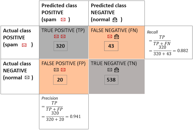
Similarly to sensitivity, recall measures how good the model is in detecting positive events. Therefore, the formula for recall is the same as for sensitivity.

Precision measures how good the model is at assigning positive events to the positive class. That is, how accurate the spam prediction is.

We divide the number of true positives by the number of all events assigned to the positive class, i.e. the sum of true positives and false positives. The precision value for the model is 0.941. Therefore, almost 95 % of the emails predicted as spam were actually spam emails.

Recall and precision are often reported pairwise because these metrics report the relevance of the model from two perspectives, also called type I error as measured by recall and type II error as measured by precision.

Recall and precision are often connected: if we use a stricter spam filter, we’ll reduce the number of dangerous emails in the inbox, but increase the number of normal emails that have to be collected from the spam box folder afterwards. The opposite, i.e. a less strict spam filter, would force us to do a second manual filtering of the inbox where some spam mails land occasionally.

Alternatively, recall and precision can be reported by a measure that combines them. One example is called F-measure, which is the harmonic mean of recall and precision:

In case of a multinomial classification model, the target column has three or more values. The emails could be labeled as “spam”, “ad”, and “normal”, for example.

Similarly to a binomial classification model, the target class values are assigned to the positive and the negative class. Here we define spam as the positive class and the normal and ad emails as the negative class. Now, the confusion matrix looks as shown in Figure 6.

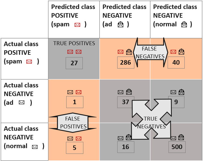
To calculate the class statistics, we have to re-define the true positives, false negatives, false positives, and true negatives using the values in a multivariate confusion matrix:

• The cell identified by the row and column for the positive class contains the True Positives, i.e. where the actual and predicted class is spam
• Cells identified by the row for the positive class and columns for the negative class contain the False Negatives, where the actual class is spam, and the predicted class is normal or ad
• Cells identified by rows for the negative class and the column for the positive class contain the False Positives, where the actual class is normal or ad, and the predicted class is spam
• Cells outside the row and column for the positive class contain the True Negatives, where the actual class is ad or normal, and the predicted class is ad or normal. An incorrect prediction inside the negative class is still considered as a true negative

Now, these four statistics can be used to calculate class statistics using the formulas introduced in the previous section.

In this article, we’ve laid the first stone for the metrics used in model performance evaluation: the confusion matrix.

Indeed, a confusion matrix shows the performance of a classification model: how many positive and negative events are predicted correctly or incorrectly. These counts are the basis for the calculation of more general class statistics metrics. Here, we reported those most commonly used: sensitivity and specificity, recall and precision, and the F-measure.

Confusion matrix and class statistics have been defined for binomial classification problems. However, we have shown how they can be easily extended to address multinomial classification problems.