Predict Demand Combining the Power of KNIME & H2O

Some time ago, we set our mind to solving a popular Kaggle challenge offered by a Japanese restaurant chain and predict how many future visitors a restaurant will receive.

Making forecasts can be a tricky business because there are so many unpredictable factors that can affect the equation; demand prediction is often based on historical data, so what happens when those data change dramatically? Will the model you are using to produce your prediction still work when the data in the real world experience change - a slow drift or a sudden jump? Who would have thought at the beginning of 2020 that restaurants around the world would soon be going into lockdown and having to come up with creative solutions to sell their products? The impact of this pandemic has brought many challenges to demand prediction because the data we are collecting now is so different to what it was before.

The data we are using to solve this Kaggle Challenge was collected during 2016 to April 2017 - so we would like to point out that it does not reflect the dramatic changes in restaurant attendances we have seen since the onset of the coronavirus pandemic.

In previous blog articles we have looked at classic demand prediction problems, for example predicting future electricity usage to shield electricity companies from power shortages or power surpluses. In this article we want to take a mixed approach to predicting how many future visitors will go out for a meal to a restaurant and also take advantage of the open architecture of KNIME Analytics Platform to bring an additional tool into the mix.

Note: We developed a cross-platform ensemble model to predict flight delays (another popular challenge). Here, cross-platform means that we trained a model with KNIME, a model with Python, and a model with R. These models from different platforms were then blended together as an ensemble model in a KNIME workflow. Indeed, one of KNIME Analytics Platform’s many qualities consists of its capability to blend data sources, data, models, and, yes, also tools.

For this restaurant demand prediction challenge we decided to develop a cross-platform solution using the combined power of KNIME Analytics Platform and H2O.

The article is split into two sections - one looks at the KNIME H2O extensions and give you information on how to instasll them. The second section is dedicated to the actual Kaggle Challenge.

• The KNIME H2O Extensions
• The Kaggle Demand Prediction Challenge

The integration of H2O in KNIME offers an extensive number of nodes and encapsulating functionalities of the H2O open source machine learning libraries, making it easy to use H2O algorithms from a KNIME workflow without touching any code - each of the H2O nodes looks and feels just like a normal KNIME node - and the workflow reaches out to the high performance libraries of H2O during execution.

There is now a new commercial offering, which joins H2O Driverless AI and KNIME Server. If this interests you, you can find more information about that here and see an example workflow on the KNIME Hub. Visit https://www.knime.com/partners/h2o-partnership.

To use H2O within KNIME Analytics Platform, all you need to do is install the relevant H2O extension and you’re ready to go. At the time of writing there are essentially two different types H2O extensions for KNIME - one type caters to big data and the other is for machine learning.

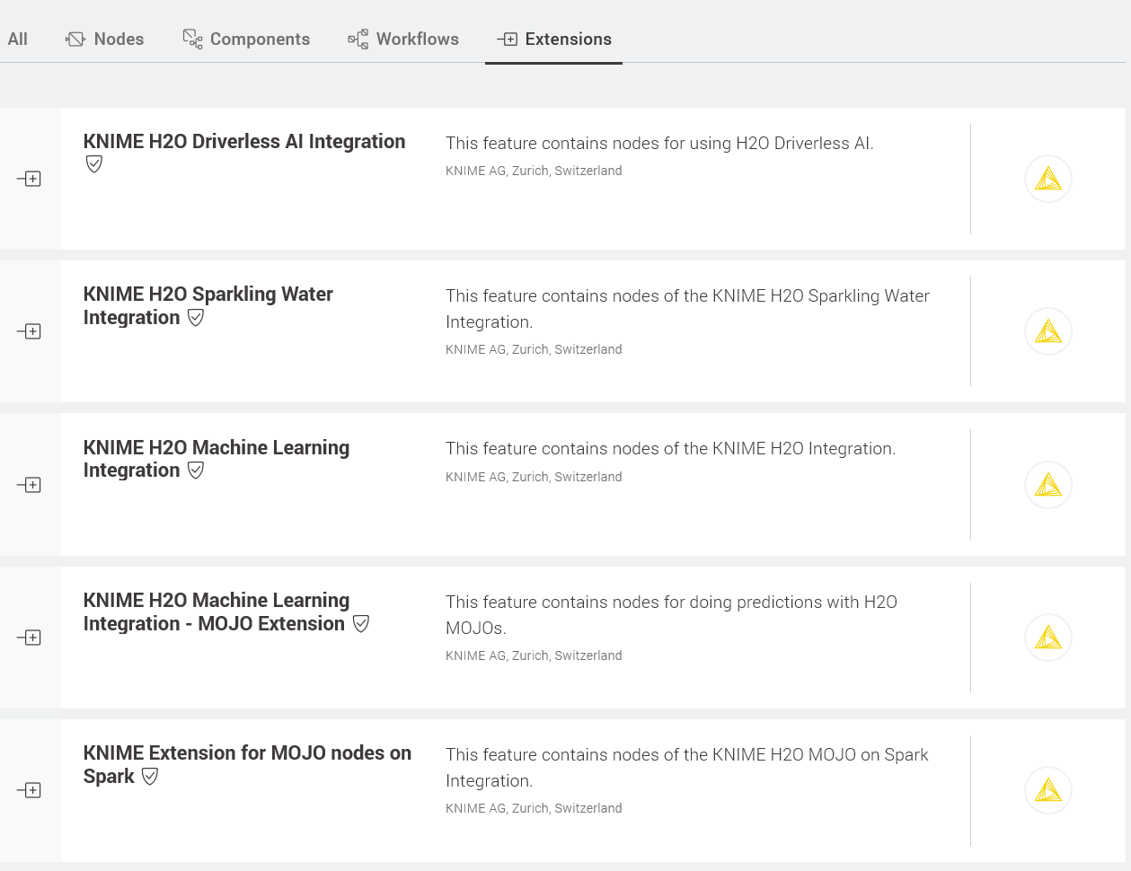
Figure 1. The KNIME H2O Extensions on the KNIME Hub.

With your installation of KNIME Analytics Platform open, go to the KNIME Hub and click the H2O extension you want to use. Next, simply drag the extension icon into the Workflow Editor. And that’s it!

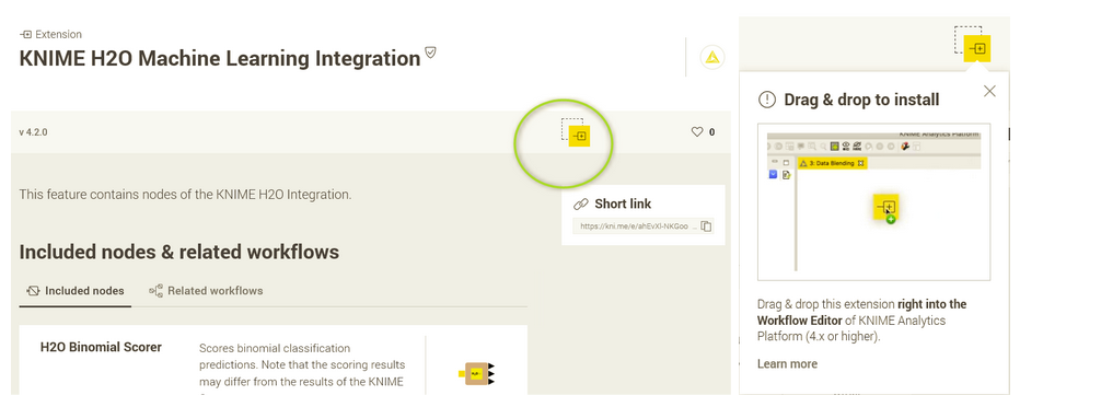
Fig. 2 The KNIME HJ2O Machine Learning Integration on the KNIME Hub - click the icon marked in green and drag and drop it to your KNIME Workflow Editor to install it.

Eight different datasets are available in this Kaggle challenge. Three of the datasets come from the so-called AirREGI (air) system, a reservation control and cash register system. Two datasets are from Hot Pepper Gourmet (hpg), which is another reservation system. A further dataset contains the store IDs from the air and the hpg systems, which allows you to join the data together, and another provides basic information about the calendar dates. At first I wondered what this might be good for, but the fact that it flags public holidays came in quite handy.

Last but not least there is a file that contains instructions for the work submission. Here, you must specify the dates and stores for your model predictions. More information on the datasets can be found at the challenge web page.

To solve the challenge, we implemented a classic best model selection framework according to the following steps:

1. Data preparation, i.e. reading, cleaning, joining data, and feature creation all with native KNIME nodes
2. Creation of a local H2O context and transformation of a KNIME data table into an H2O frame
3. Training of three different H2O based Machine Learning models (Random Forest, Gradient Boosted Machine, Generalized Linear Models). Training procedure also includes cross-validation and parameter optimization loops, by mixing and matching native KNIME nodes and KNIME H2O extension nodes.
4. Selection of the best model in terms of RMSLE (Root Mean Squared Logarithmic Error) as required by the Kaggle Challenge.
5. Deployment, i.e. converting the best model into an H2O MOJO (Model ObJect Optimized) object and running it on the test data to produce the predictions to submit to the Kaggle competition.

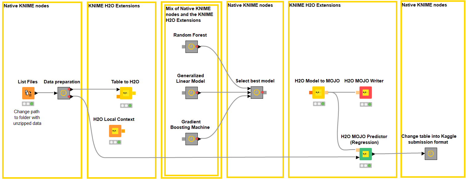
Fig. 3. The KNIME workflow, Customer Prediction with H2O, implemented as a solution to the Kaggle restaurant competition. Notice the mix of native KNIME nodes and KNIME H2O extension nodes. The KNIME H2O Machine Learning Integration extension nodes encapsulate functionalities from the H2O library.

Let’s now take a look at these steps one by one.

The workflow starts by reading seven of the datasets available on the Kaggle challenge page.

The metanode named “Data preparation” includes flagging weekend days vs. business days; joining reservation items; aggregating (mean, max, and min) on groups of visitors, as by restaurant genre and/or geographical area.

The dataset contains a column indicating the number of visitors for a particular restaurant on a given day. This value will be used as the target variable to train the predictive models later on in the workflow. At the end of the data preparation phase, the dataset is then split in two parts: one part with the rows with a non-missing value for the field “number of visitors” and one part containing the remaining records with missing number of visitors. The last dataset represents the test set upon which the predictions will be calculated to submit to the Kaggle competition.

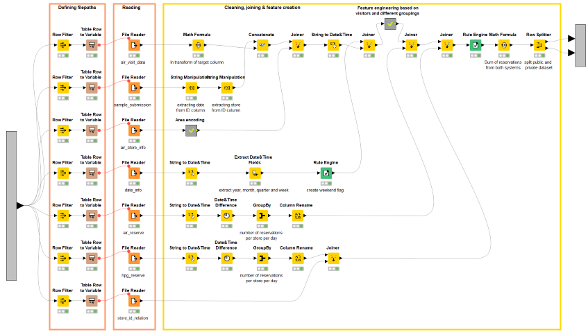
Fig. 4. This is the sub-workflow contained in the “Data preparation” metanode. It implements weekend vs. business day flagging, data blending via joining, as well as a few aggregations by restaurant group.

As you can see from the screenshot in Figure 4, the data processing part was implemented solely with native KNIME nodes, so as to have a nicely blended, feature enriched dataset in the end.

To be able to use the H2O functionalities, you need to start an H2O environment. The H2O Local Context node does the job for you. Once you’ve created the H2O context, you can convert data from your KNIME data tables into H2O frames and train H2O models on these data.

As the prediction problem was a regression task, I chose to train the following H2O models: Random Forest, Generalized Linear Model, and Gradient Boosting Machine algorithm.

The H2O models were trained and optimized inside the corresponding metanodes in Figure 1. Let’s take a look for example at the metanode named “Gradient Boosting Machine” (Fig. 4). Inside the metanode you’ll see the classic Learner-Predictor motif, but this time the two nodes rely on H2O based code. The “Scoring (RMSLE)” metanode calculates the error measure. We repeat this operation five times using a cross-validation framework.

The cross-validation framework is interesting. It starts with an H2O node - H2O Cross-Validation Loop Start node - and it ends with a native KNIME Loop End node. The H2O Cross-Validation Loop Start node implements the H2O cross-validation procedure extracting a random different validation subset at each iteration. The Loop End node collects the error measure from each cross-validation result. The two nodes blend seamlessly, even though they refer to two different analytics platforms.

On top of all that, an optimization loop finds the optimal parameters of the specific model for the smallest RMSLE average error. This loop here is completely controlled via native KNIME nodes. The best parameters are selected via the Element Selector node and the model is trained again on all training data with the optimal parameters.

As you can see, the mix and match of native KNIME nodes and H2O functionalities is not only possible, but actually quite easy and efficient.

Fig. 5. Content of the “Gradient Boosting Machine” metanode , including model training and model prediction, cross-validation loop, and optimization loop. Notice the H2O Cross-validation Loop Start node blends seamlessly with the native KNIME Loop End node.

As a result of the previous step I have a table with three different models with their respective RMSLE scores, as this is the metric used by Kaggle to compute the leaderboard. RSMLE was likely chosen over root mean squared error due to its robustness to outliers and the fact that it penalizes underestimations stronger than overestimations, i.e. by optimizing your model for RMSLE you rather plan with more customers than actually visiting your restaurant.

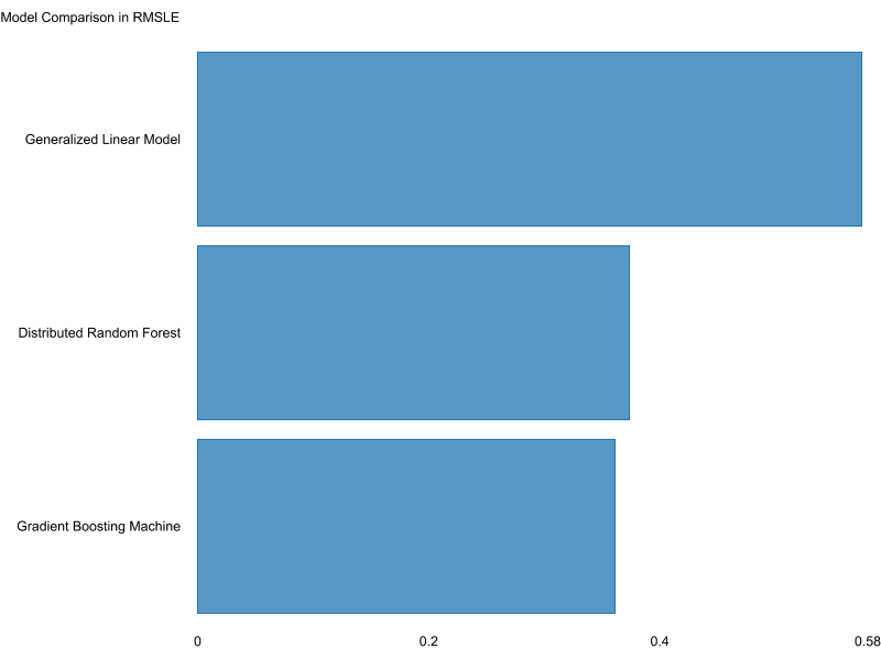
Fig. 6. Bar chart comparing scores of the three different models. Y-axis shows the model names and x-axis shows their score in RMSLE.

From the chart one can easily see that Random Forest and Gradient Boosting Machine outperformed Generalized Linear Model in this case. Random Forest and GBM almost end up in a tie, GBM only having a slightly lower RMSLE. Our workflow automatically selects the model that scored best with the Element Selector node, in the metanode named “Select best model”.

Afterwards the model is transformed into an H2O MOJO (Model ObJect, Optimized) object. This step is necessary in order to use an H2O model outside of an H2O context and to use the general H2O MOJO Predictor node.

Remember that the blended dataset was split in two partitions? The second partition, without the number of visitors, is the submission dataset. The MOJO model that was just created is applied to the submission dataset. The submission dataset, this time with predictions, is then transformed into the required Kaggle format and sent to Kaggle for evaluation.

• You can download the final workflow, Customer Prediction with H2O in KNIME from the KNIME Hub.

We did it! We built a workflow to solve the Kaggle challenge.

The workflow blended native KNIME nodes and KNIME H2O Extension nodes, thus combining the power of KNIME Analytics Platform and H2O under the same roof.

The mix and match operation was the easiest part of this whole project. Indeed, both the KNIME and H2O open source platforms have proven to work well together, complementing each other nicely.

We built this workflow not with the idea of winning (the submission deadline was over before we even got our hands on this anyway), but to showcase the openness of KNIME Analytics Platform and how easily and seamlessly the KNIME H2O extension integrates H2O in a KNIME workflow. The workflow indeed can still be improved, maybe with additional machine learning models - that would potentially be able to cope with factors such as the change in data that we are experiencing due to the COVID-19 pandemic - with more sophisticated feature engineering, or with the adoption of an ensemble model rather than of the best selected model.

Well now, would you like to know how we scored on Kaggle? Our submission had a RMSLE of 0.515, which puts it in the top 3% of more than 2000 submissions. Considering that we spent just a few days on this project, we are quite satisfied with this result.