Teradata Aster meets KNIME Table: Will They Blend?

In this blog series we’ll be experimenting with the most interesting blends of data and tools. Whether it’s mixing traditional sources with modern data lakes, open-source devops on the cloud with protected internal legacy tools, SQL with noSQL, web-wisdom-of-the-crowd with in-house handwritten notes, or IoT sensor data with idle chatting, we’re curious to find out: will they blend? Want to find out what happens when IBM Watson meets Google News, Hadoop Hive meets Excel, R meets Python, or MS Word meets MongoDB?

Today’s challenge is related to the healthcare industry. You know that little pain in the chest you sometimes feel and you do not know whether to run to the hospital or just wait until it goes away? Would it be possible to recognize as early as possible just how serious an indication of heart disease that little pain is?

The goal of this experiment is to build a model to predict whether or not a particular patient with that chest pain has indeed heart disease.

To investigate this topic, we will use open-source data obtained from the University of California Irvine Machine Learning Repository, which can be downloaded from http://archive.ics.uci.edu/ml/machine-learning-databases/heart-disease/. Of all datasets contained in this repository, we will use the processed Switzerland, Cleveland, and VA data sets and the reprocessed Hungarian data set.

These data were collected from 920 cardiac patients: 725 men and 193 women aged between 28 and 77 years old; 294 from the Hungarian Institute of Cardiology, 123 from the University Hospitals in Zurich and Basel, Switzerland, 200 from the V.A. Medical Center in Long Beach, California, and 303 from the Cleveland Clinic in Ohio.

Each patient is represented through a number of demographic and anamnestic values, angina descriptive fields, and electrocardiographic measures (http://archive.ics.uci.edu/ml/machine-learning-databases/heart-disease/heart-disease.names).

In the dataset each patient condition is classified into 5 levels according to the severity of his/her heart disease. We simplified this classification system by transforming it into a binary class system: 1 means heart disease was diagnosed, 0 means no heart disease was found.

This is not the first time that we are running this experiment. In a not even that remote past, we built a Naïve Bayes KNIME model on the same data to solve the same problem. Today we want to build a logistic regression model and see if we get any improvements on the Naïve Bayes model performance.

Original patient data are stored in a Teradata database. The predictions from the old Naïve Bayes model are stored in a KNIME Table.

Teradata Aster is a proprietary database system that may be in use at your company/organization. It is designed to enable multi-genre advanced data transformation on massive amounts of data. If your company/organization is a Teradata Aster customer, you can obtain the JDBC driver that interfaces with KNIME by contacting your company’s/organization’s Teradata Aster account executive.

Table format is a KNIME proprietary format to store data efficiently, in terms of size and retrieval speed, and completely, i.e. also including their structure metadata. This leads to smaller local files, faster reading, and minimal configuration settings. In fact, the Table Reader node, which reads such Table files, only needs the file path and retrieves all other necessary information from the metadata saved in the file itself. Files saved in KNIME Table format carries an extension “.table”.

Teradata Aster on one side, KNIME Table formatted file on the other side. The question, as usual, is: Will they blend? Let’s find out.

Topic. Predicting heart disease. Is this chest pain innocuous or serious?

Challenge. Blend data from Teradata Aster system with data from a KNIME .table file. Build a predictive model to establish presence or absence of heart disease.

Access Mode. Database Connector node with Teradata JDBC driver to retrieve data from Teradata database. Table Reader node to read KNIME Table formatted files.

Accessing the Teradata Aster database

1. First of all, we needed the appropriate JDBC driver to interface Teradata Aster with KNIME. If your company/organization is a Teradata Aster customer, the noarch-aster-jdbc-driver.jar file can be obtained by contacting your Teradata Aster account executive.
2. Once we downloaded the noarch-aster-jdbc-driver.jar file, we imported it into the list of available JDBC drivers in KNIME Analytics Platform.
   1. Open KNIME Analytics Platform and select File -> Preferences -> KNIME -> Databases -> Add File.
   2. Navigate to the location where you saved the noarch-aster-jdbc-driver.jar file.
   3. Select the .jar file, then click Open -> OK.
3. In a KNIME workflow, we configured a Database Connector node with the Teradata Aster database URL (<protocol> = jdbc:ncluster), the just added JDBC driver (com.asterdata.ncluster.jdbc.core.NClusterJDBCDriver) and the credentials to the same Teradata Aster database.
4. The Database Connector node was then connected directly to a Database Reader node. Since we are quite expert SQL coders, we implemented the data pre-processing into the database Reader node in the form of SQL code. The SQL code selects the [schema].heartdx_prelim table, creates an ID variable called “rownum” (without quotes) and the new binary response variable, named dxpresent, (disease =1, no disease=0), and recodes missing values (represented by -9s and, for some variables, 0s) as true NULL values. The SQL code is shown below:
   

   DROP TABLE IF EXISTS [schema].knime_pract;
    
   CREATE TABLE [schema].knime_pract 
   DISTRIBUTE BY HASH(age)
   COMPRESS LOW AS (
       SELECT
        (ROW_NUMBER() OVER (ORDER BY age)) AS rownum,
        age,
            gender,
        chestpaintype,
        CASE
            WHEN restbps = 0 THEN null
            ELSE restbps
            END AS restbps,
            CASE
            WHEN chol = 0 THEN null
            ELSE chol
            END AS chol,
            fastbloodsug, 
            restecg,
            maxheartrate, 
            exindang,
            oldpeak,
            slope,
            numvessels,
            defect,
            dxlevel,
            CASE
            WHEN dxlevel IN ('1', '2', '3', '4') THEN '1'
            ELSE '0'
            END AS dxpresent
       FROM [schema].heartdx_prelim
   );
    
   SELECT * FROM [schema].knime_pract;
   

If you are not an expert SQL coder, you can always use the KNIME in-database processing nodes available in the Node Repository in the Database/Manipulation sub-category.

Building the Predictive Model to recognize possible heart disease

1. At this point, we have imported the data from the Teradata Aster database into our KNIME workflow. More pre-processing, however, was still needed:
   1. Filtering out empty or almost empty columns; that is, columns with too many missing values (please see this article for tips on dimensionality reduction: https://www.knime.org/blog/seven-techniques-for-data-dimensionality-reduction)
   2. On the remaining columns, performing missing value imputation in a Missing Value node by replacing missing numeric values (both long and double) with the median and missing string values with the most frequently occurring value
   3. Partitioning the dataset into training and test set using a Partitioning node (80% vs. 20%)
2. After this pre-processing has been executed, we can build the predictive model. This time we chose a logistic regression model. A Logistic Regression Learner node and a Regression Predictor node were been introduced into the workflow.
   1. Column named dxpresent was used as the target variable in the Logistic Regression Learner node.
   2. Box “Append columns…” was checked in the Regression Predictor node. This last option is necessary to produce the prediction values which will later be fed into an ROC Curve node to compare the 2 models performances.

Reading data from the KNIME .table file

Here we just needed to write the Table file path into a Table Reader node. Et voilà we got the predictions previously produced by a Naïve Bayes model.

Note. The file path is indeed all you need! All other necessary information about the data structure is stored in the .table file itself.

Blending Predictions

1. After training the logistic regression model, we used a Joiner node to connect its predictions to the older predictions from the Naïve Bayes model.
2. We then connected an ROC Curve node, to display the false positives and true positives, through P(dxpresent=1), for both models.

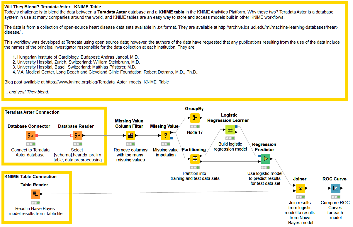
The final workflow is shown in figure 1 and it is available for download on the EXAMPLES server under 01_Data_Access/02_Databases/09_Teradata_Aster_meets_KNIME_Table01_Data_Access/02_Databases/09_Teradata_Aster_meets_KNIME_Table^*.

Figure 1. This workflow retrieves data from a Teradata Aster database, builds a predictive model (Logistic Regression) to recognize the presence of a heart disease, blends this model’s predictions with the predictions of an older model (Naïve Bayes) stored in a KNIME Table file, and then compares the 2 models performances through an ROC curve.

(click on the image to see it in full size)

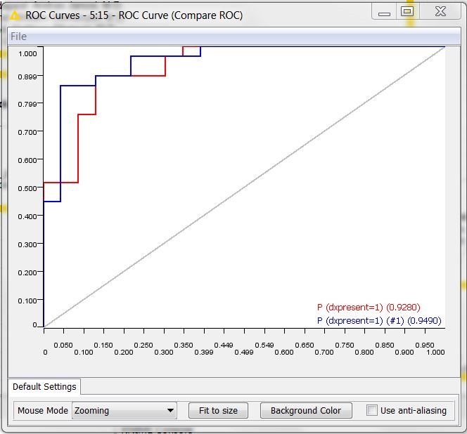
The ROC curves resulting from the workflow are shown in figure 2. The red curve refers to the logistic regression, the blue curve to the old Naïve Bayes model. We can see that the Naïve Bayes model, though being older, is not obsolete. In fact, it shows an area under the curve (0.95) comparable to the area under the curve of the newer logistic regression (0.93).

Figure 2. ROC curves of the Logistic Regression (in red) and of the old Naive Bayes model (in blue)

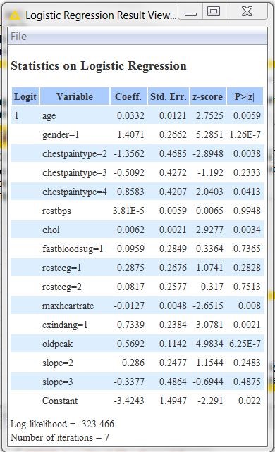
To conclude, let’s spend two words on the logistic regression model interpretation. After opening the view of the Logistic Regression node, we get the table in figure 3. There, from the coefficient values you can see that gender and chest pain type #2 (atypical angina) are the main drivers for the prediction, although patients with chest pain type #2 are less likely to have heart disease than those with other types of chest pain.

Are men more affected than women by heart disease? Does this describe a general a priori probability or is it just the a priori probability of the data set? It would be interesting here to see how many men with chest pain = 2 have heart disease and how many do not. Same for women. We can investigate this with a GroupBy node following the Missing Value node. We configure the GroupBy node to group data rows by gender, chest pain type, and dxpresent; our desired aggregation is the count of the number of rows (on rownum column).

After execution, we find that 60 out of 193 women have chest pain type #2; of the women with this chest pain type, 4 have heart disease while 56 do not. In other words, our data set shows that women with chest pain type #2 have only a 4/60 = 6.7% chance of having heart disease. For the men, we find that 113 out of 725 men have chest pain type #2; of the men with this type of chest pain, 20 have heart disease while 93 do not. According to our data, men with chest pain type #2 have a 20/113 = 17.7% chance of having heart disease.

Figure 3. Coefficients of the Linear Regression model to predict presence/absence of heart disease

In this experiment we have successfully blended predictions from a logistic regression model trained on data stored in a Teradata database with older predictions from a Naïve Bayes model stored in a KNIME Table formatted file.

Again, the most important conclusion of this experiment is: Yes, they blend!

If you enjoyed this, please share this generously and let us know your ideas for future blends.

We’re looking forward to the next challenge. What about blending SQL dialects? For example one of the many Hadoop Hive SQL dialects and Spark SQL. Will they blend?

---

The authors of the databases have requested that any publications resulting from the use of the data include the names of the principal investigator responsible for the collection of the data at each institution. They would be:

1. Hungarian Institute of Cardiology. Budapest: Andras Janosi, M.D.
2. University Hospital, Zurich, Switzerland: William Steinbrunn, M.D.
3. University Hospital, Basel, Switzerland: Matthias Pfisterer, M.D.
4. V.A. Medical Center, Long Beach and Cleveland Clinic Foundation: Robert Detrano, M.D., Ph.D.

* The link will open the workflow directly in KNIME Analytics Platform (requirements: Windows; KNIME Analytics Platform must be installed with the Installer version 3.2.0 or higher)