Analyzing Gene Expression Data with KNIME

All individuals are unique and so are our data needs. From simple csv files to REST APIs to Google’s BigQuery or using customized shared components, KNIME Analytics Platform offers many ways to access and analyze your data. Today, we will demonstrate how to access all of these aforementioned data sources through the use case of analyzing and annotating gene expression data.

Gene expression analysis is widely used in bioinformatics because it enables researchers to find gene products with increased or decreased synthesis in individuals with e.g. particular diseases. Gene expression is the process by which information from a gene is used in the synthesis of a functional gene product.

As we learned in a recent blog article, Motifs and Mutations - The Logic of Sequence Logos, DNA mutations yield different effects of varying impact. Some have no noticeable effect at all and some can lead to severe diseases. As we also saw in that blog post, mutations that change gene expression are often associated with harmful effects. Hence, analyzing gene expression data directly is a straightforward way to find connections between genes and diseases.

The first step in gene expression is called transcription, during which DNA is transcribed to RNA. Advances in massively parallel sequencing enable the rapid sequencing of this RNA (RNA-Seq) in a genome-wide manner in order to quantify the amount of synthesized gene product.

In our use case today we:

• Analyze RNA-Seq data from tumors and matched normal tissue from three patients with oral squamous cell carcinomas¹
• Investigate all statistically significant over/under expressed genes and select interesting ones by looking into their functional annotations.
• Using hierarchical clustering, we select a cluster of similarly expressed genes and investigate their pathway enrichment.
• Search for compounds that target the gene products we picked.

As illustrated in Figure 1, the overall workflow, Gene Expression Analysis, which can be downloaded from the KNIME Hub, consists of the following steps:

1. Input data
2. Find differentially expressed genes
3. View results of differential gene expression analysis
4. Clustering
5. Pathway enrichment
6. Display compounds targeting gene product of interest

Figure 1. Overview of workflow. Differentially expressed genes are discovered using R and then displayed in an interactive view. Subsequently, genes are hierarchically clustered based on their expression pattern, and the results are shown via a dendrogram alongside a heatmap. We then perform a pathway enrichment analysis and look for compounds targeting the gene product of interest.

The user can select the files containing RNA-Seq data for samples with and without a disease of interest (positive and control, respectively). This data then gets used in the R Snippet to find differentially expressed genes. The user can investigate those genes and select genes of interest based on statistics from the gene expression analysis. We then cluster the genes based on similar expression profiles and investigate their biological pathways. In the last step we search for compounds targeting the selected gene products.

As mentioned in the previous section, today’s example uses RNA-Seq data from normal and tumor cells from patients with oral squamous cell carcinomas². The standard procedure to generate that data consists of the following steps: the RNA of the cells is reversely transcribed to cDNA and then sequenced using massively parallel sequencing resulting in short sequenced reads. Subsequently, these reads are mapped back to the reference genome to identify the genes from which they originated. This results in a count for each position in a gene representing the amount of gene product. In our data set, read counts for 10,542 genes were collected.

One of the strengths of KNIME Analytics Platform lies in its openness for other tools. This allows you to easily harness the power of those tools such as R with all of its libraries. In our case today we want to utilize a commonly used R library for differential expression analysis of RNA-seq expression profiles: edgeR³. EdgeR implements a range of statistical methods including likelihood tests based on generalized linear models (GLM). GLMs are most commonly used to model binary or count data which makes them perfectly suited to model the aforementioned read counts. GLMs model a response by a linear function of explanatory variables and allow for constraints such as a restriction on the range of the response Y or the variance of Y depending on the mean. Hence, a generalized linear model is made up of three components: (1) a linear predictor, (2) a link function that describes how the mean depends on the linear predictor and (3) a variance function that describes how the variance depends on the mean [var(Yi) =φV(μ), with φ being the dispersion parameter].

Therefore, in our R snippet, we use the read count data from tumor vs. normal tissue and estimate the dispersion parameter. In the next step, we fit the generalized linear model and apply a likelihood-ratio test. This results in a log fold-change (logFC) and a p-value for each gene. The logFC describes how much a quantity changes between an original and a subsequent measurement. In our case that means how much the read counts per gene differ between tumor and normal cells. As we do this simultaneously for all 10,542 genes, we have to make sure to apply a multiple testing correction⁴. We use the default method provided by edgeR, Benjamini-Hochberg, which has the false discovery rate (FDR) as output.

As we are interested in the relative changes in expression levels between conditions, we do not have to account for factors such as varying gene length. However, we have to account for differing sequencing depth and RNA composition. Sequencing depth is adjusted in edgeR as part of the basic modeling procedure. To adjust for RNA composition effects, where highly expressed genes can cause the remaining genes to be under-sampled in that sample, we use the function calcNormFactors. In addition to the fold-change and the FDR for each gene, we extract the depth-normalized read counts (counts-per-million) for each gene in our analysis.

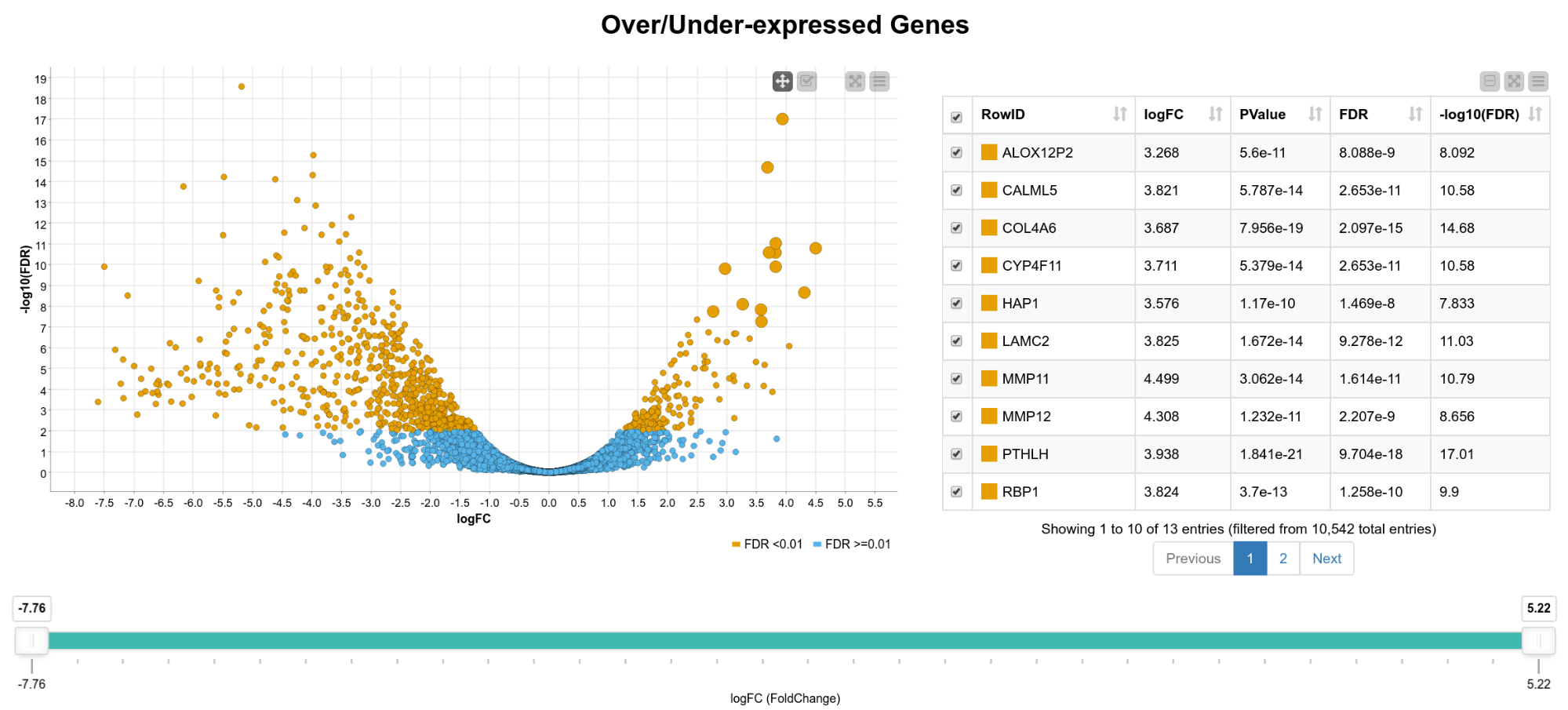
We now have statistics for 10,542 genes, so in the following steps we want to narrow down the results to genes of interest. For that, we create an interactive composite view in which the user can select genes for further analysis. As can be seen in Figure 2, we display the fold-change vs. the FDR on a logarithmic scale in a scatter plot. The colors indicate if the FDR exceeds 0.01 or not. In addition, we show an interactive table with details of the results (FDR, -log10(FDR) , p-value, gene name) and a range slider that allows the user to interactively filter for the logFC. We can now, for example, extract only genes that are significantly upregulated in tumor cells by box selecting the genes in the upper right corner of the scatter plot.

Figure 2. View of differentially expressed genes. A scatter plot of the fold change vs. the FDR and a table with details of the result is shown. The user can select genes in the plot, the table, or filter by fold change using the range slider.

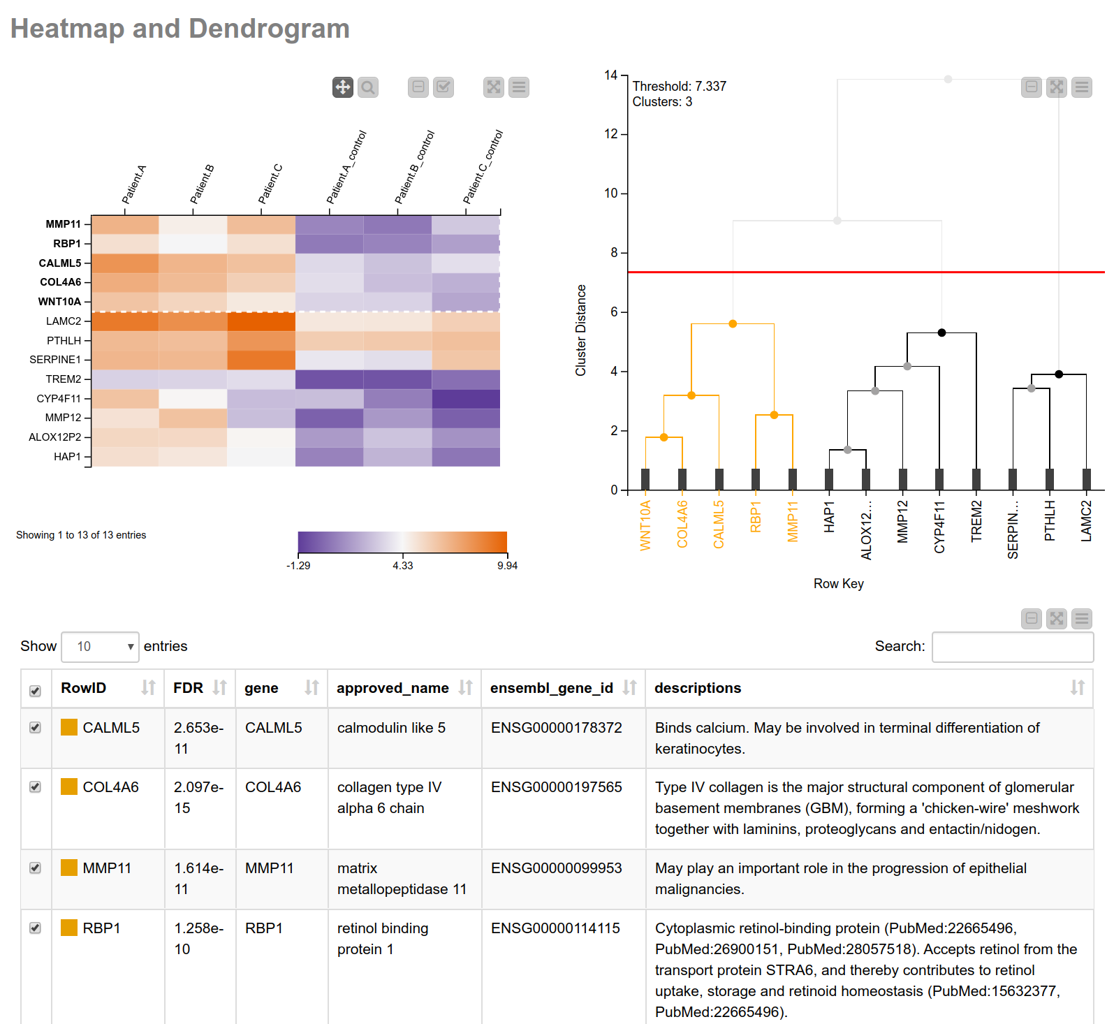
Having narrowed down our search space, let’s have a closer look into the biological processes associated with these genes. Similar expression patterns of genes often point to a common function⁵. To find those genes with similar expression patterns, we perform a hierarchical clustering on the normalized read counts and display the results in a hierarchical cluster tree. For this, we can use a shared component that can be found on the KNIME Hub, the component Hierarchical Clustering and Heatmap. This component allows you to perform a hierarchical clustering on numerical columns of your choice and to display a heatmap sorted according to the clustering results. We combine this component with a table containing more detailed information about the genes (see Fig. 3), allowing us to interactively identify and pick a cluster of interest. In our case we select the one showing high (orange) values in tumor cells and low (blue) values in the matched normal tissue. As we can learn from the details in the table of our composite view, this cluster includes MMP11 (matrix metallopeptidase 11) which may play an important role in the progression of epithelial malignancies, and COL4A6 (collagen type IV alpha 6 chain) which is the major structural component of glomerular basement membranes.

To further investigate shared function of the selected genes we perform a pathway enrichment analysis in the next step.

Figure 3. View of heatmap with normalized read counts and dendrogram showing the hierarchical clustering of the counts. The heatmap is sorted according to the clustering. This combination of the heatmap with the dendrogram can be easily achieved using the shared component “Hierarchical Clustering and Heatmap”. Additionally, a table with more detailed information is shown.

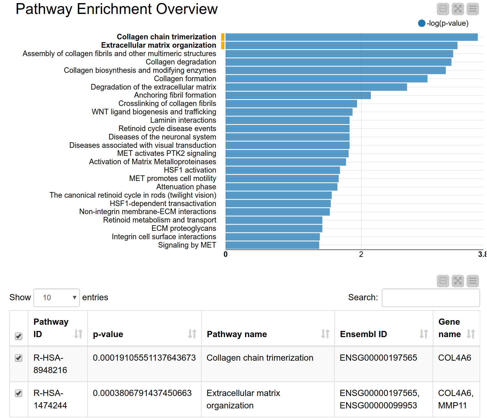
A pathway consists of a set of genes related to a specific biological function. As genes are often annotated to a lot of pathways, a pathway enrichment analysis allows us to find those pathways that are enriched in the input set of genes more than would be expected by chance⁶. Pathway enrichment analysis is, therefore, a widely used tool for gaining insight into the underlying biology of differentially expressed genes, as it reduces complexity and has increased explanatory power⁷. Again, we can use the KNIME hub to easily drag and drop a shared component called Pathway Enrichment Analysis. This component makes use of the Reactome Pathway Database, a resource which is open-source, curated and peer-reviewed. It provides a pathway enrichment web service which can be easily accessed by KNIME Analytics Platform. The component takes as input a set of Ensembl gene IDs and automatically performs the pathway enrichment analysis, the results can be seen in Figure 4. The pathways with the most significant enrichment are “Collagen chain trimerization” and “Degradation of the extracellular matrix”. Both MMP11 and COL4A6 are part of these two pathways. Indeed, collagen is an essential part of the extracellular matrix and extracellular matrix interactions are known to be involved in the process of tumor invasion and metastasis in oral squamous carcinoma⁸. This further corroborates our hypothesis that these genes play an important role in oral squamous cell carcinomas from our patients’ tumor cells.

Figure 4. Pathway enrichment view. The pathways with the highest enrichment are “Collagen chain trimerization” and “Degradation of the extracellular matrix”.

In this final step, we want to check if we can possibly interfere with the disease for which we did our expression data analysis. For that, we look for compounds that target the selected gene products. As we have seen in a previous blog article Interactive exploration and analysis of scientific datasets using Google BigQuery and KNIME Analytics Platform, Google BigQuery offers effortless access to public life sciences data. For this, you need to set up a BigQuery Account first, you can find more details on how to do that in this blog article: Tutorial - Importing Bike Data from GoogleBigquery. In particular, we can easily query bioactivity data from the database ChEMBL using the KNIME Google BigQuery Connector in combination with the KNIME Database nodes. For our query we gather all human synonyms for the gene products of choice and extract compounds known to target those. This allows us to retrieve information for all those compounds including the name, the assay ID, the type of measurement (e.g. IC50 or Ki), and the structure as SMILEs string.

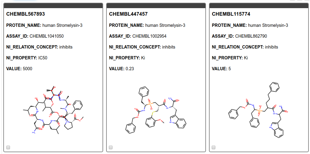
From the SMILES string we create images of the molecules and display them in a tile view. As can be seen in Figure 5 we found only results for MMP11, Matrix metalloproteinase-11 also known as Stromelysin-3. MMP11 is known to be involved in extracellular matrix breakdown in normal physiological processes and has been implicated in promoting cancer development by inhibiting apoptosis as well as enhancing migration and invasion of cancer cells⁹. Additionally, it has been revealed that MMP-11 expression in oral squamous cell carcinoma samples can predict the progression and the survival of oral squamous cell carcinoma patients¹⁰. Moreover, MMP11 has been recently been identified as potential therapeutic target in lung adenocarcinoma. ¹¹

Figure 5. Tile view with compounds targeting the gene product of interest. The ChEMBL ID for the ligand, the name of the target, the assay ID, the action, the type of measurement, and its value are shown.

Today we learned how to perform a classic task in bioinformatics: differential gene expression analysis for a disease of interest. We created an interactive view that allowed the user to select significantly under/over expressed genes. From there we further narrowed that set of genes down to genes with similar expression patterns and common function. In the last step, we searched for compounds targeting the discovered gene products thereby offering the possibility to interfere with the disease under investigation. We applied our workflow to data from normal and tumor cells from patients with oral squamous cell carcinoma. Through our analysis we were able to identify a gene that has been independently implicated as a therapeutic target for carcinomas. Moreover, it has been shown that the expression of that gene can predict disease progression as well as survival of oral squamous cell carcinoma patients. All this was facilitated by KNIME’s openness for other tools which enabled us to use our favourite R library, extract data from Google’s BigQuery and use shared components to customize our analysis.

All steps of the analysis can also be performed on the WebPortal through the interactive views of the components.

• The workflow Gene Expression Analysis used for this blog post can be downloaded from the KNIME Hub at this link: https://kni.me/w/vUgr-iyGudXur-1B

Download this innovation note as a PDF

References

^1. Tuch, B., Laborde, R., Xu, X., Gu, J., Chung, C., & Monighetti, C. et al. (2010). Tumor Transcriptome Sequencing Reveals Allelic Expression Imbalances Associated with Copy Number Alterations. Plos ONE, 5(2), e9317. doi: 10.1371/journal.pone.0009317

^2. Tuch, B., Laborde, R., Xu, X., Gu, J., Chung, C., & Monighetti, C. et al. (2010). Tumor Transcriptome Sequencing Reveals Allelic Expression Imbalances Associated with Copy Number Alterations. Plos ONE, 5(2), e9317. doi: 10.1371/journal.pone.0009317

^3. Robinson, M., McCarthy, D., & Smyth, G. (2009). edgeR: a Bioconductor package for differential expression analysis of digital gene expression data. Bioinformatics, 26(1), 139-140. doi: 10.1093/bioinformatics/btp616

^4. Noble, W. (2009). How does multiple testing correction work?. Nature Biotechnology, 27(12), 1135-1137. doi: 10.1038/nbt1209-1135

^5. Alon, U., Barkai, N., Notterman, D., Gish, K., Ybarra, S., Mack, D., & Levine, A. (1999). Broad patterns of gene expression revealed by clustering analysis of tumor and normal colon tissues probed by oligonucleotide arrays. Proceedings Of The National Academy Of Sciences, 96(12), 6745-6750. doi: 10.1073/pnas.96.12.6745

^6. Reimand, J., Isserlin, R., Voisin, V. et al. Pathway enrichment analysis and visualization of omics data using g:Profiler, GSEA, Cytoscape and EnrichmentMap. Nat Protoc 14, 482–517 (2019). https://doi.org/10.1038/s41596-018-0103-9

^7. Khatri P, Sirota M, Butte AJ (2012) Ten Years of Pathway Analysis: Current Approaches and Outstanding Challenges. PLoS Comput Biol 8(2): e1002375. https://doi.org/10.1371/journal.pcbi.1002375

^8. Lyons, A., & Jones, J. (2007). Cell adhesion molecules, the extracellular matrix and oral squamous carcinoma. International Journal Of Oral And Maxillofacial Surgery, 36(8), 671-679. doi: 10.1016/j.ijom.2007.04.002

^9. ZHANG, X., HUANG, S., GUO, J., ZHOU, L., YOU, L., ZHANG, T., & ZHAO, Y. (2016). Insights into the distinct roles of MMP-11 in tumor biology and future therapeutics (Review). International Journal Of Oncology, 48(5), 1783-1793. doi: 10.3892/ijo.2016.3400

^10. Hsin, C., Chou, Y., Yang, S., Su, S., Chuang, Y., Lin, S., & Lin, C. (2017). MMP-11 promoted the oral cancer migration and FAK/Src activation. Oncotarget, 8(20). doi: 10.18632/oncotarget.15824

^11. Yang, H., Jiang, P., Liu, D., Wang, H., Deng, Q., & Niu, X. et al. (2019). Matrix Metalloproteinase 11 Is a Potential Therapeutic Target in Lung Adenocarcinoma. Molecular Therapy - Oncolytics, 14, 82-93. doi: 10.1016/j.omto.2019.03.012