In a previous blog post, I discussed visualizations in KNIME Analytics Platform. Having recently moved to Berlin, I have been paying more attention to street graffiti. So today, we will be learning how to tag.
...just kidding. Sort of.
Our focus will be on tagging, but the text-mining (rather than street art) variety: We will learn how to automatically tag disease names in biomedical literature.
Introduction
The rapid growth in the amount of biomedical literature becoming available makes it impossible for humans alone to extract and exhaust all of the useful information it contains. There is simply too much there. Despite our best efforts, many things would fall through the cracks, including valuable disease-related information. Hence, automated access to disease information is an important goal of text-mining efforts1. This enables, for example, the integration with other data types and the generation of new hypotheses by combining facts that have been extracted from several sources2.
In this blog post, we will use KNIME Analytics Platform to create a model that learns disease names in a set of documents from the biomedical literature. The model has two inputs: an initial list of disease names and the documents. Our goal is to create a model that can tag disease names that are part of our input as well as novel disease names. Hence, one important aspect of this project is that our model should be able to autonomously detect disease names that were not part of the training.
To do this, we will automatically extract abstracts from PubMed and use these documents (the corpus) to train our model starting with an initial list of disease names (the dictionary). We then evaluate the resulting model using documents that were not part of the training. Additionally, we test whether the model can extract new information by comparing the detected disease names to our initial dictionary.
Subsequently, we interactively inspect the diseases that co-occur in the same documents and explore genetic information associated with these diseases.
Our workflow has three main parts (see Fig 1.), which will be described in detail in the following:
- Dictionary and Corpus Creation
- Model Training and Evaluation
- Co-occurrence of Tagged Disease Names
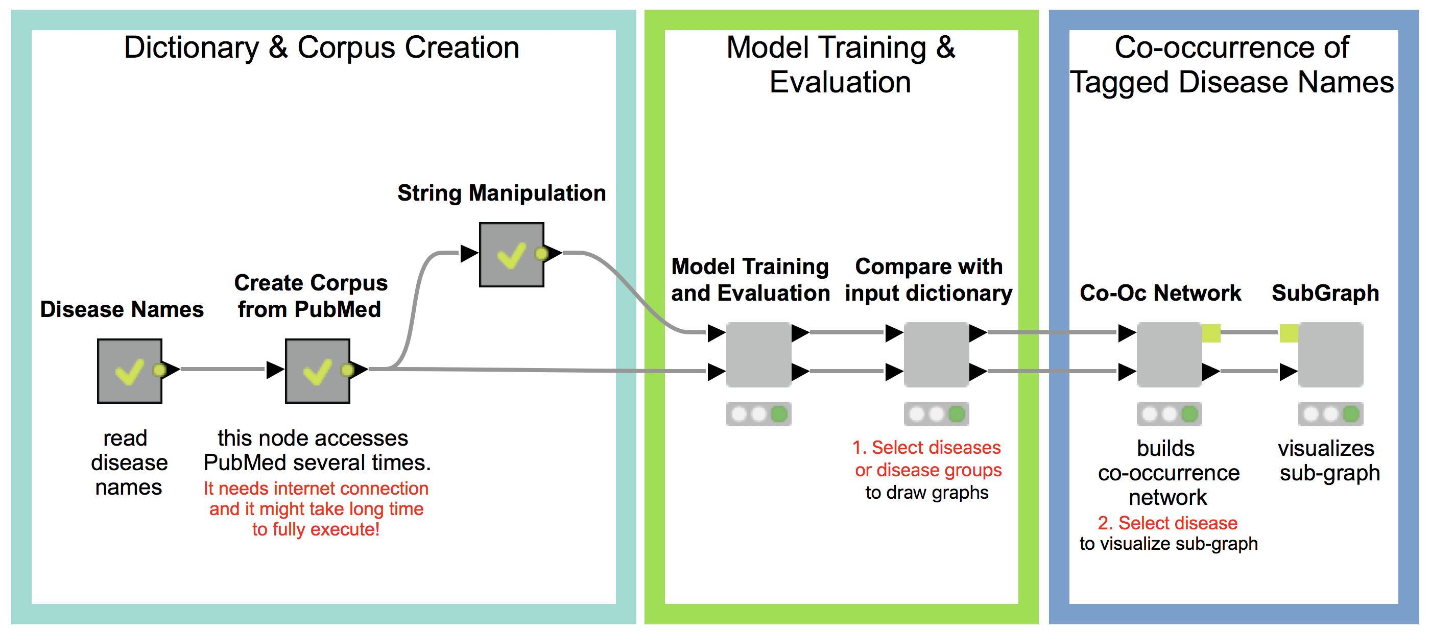
1. Dictionary and Corpus Creation
Dictionary creation (Disease Names)
For the initial input, we create a dictionary that contains disease names from Ensembl Biomart. For that, we downloaded phenotypes (diseases and traits) that are associated to genes or variants. These diseases and traits are assembled from different sources such as OMIM, Orphanet, and DDG2P. To create a dictionary that contains commonly used disease names, we filter the documents for disease names that are contained in at least three sources. The model we eventually train is case sensitive, thus, we add variations such as capitalizing the disease names, lowercase, and uppercase. The resulting disease names comprise our initial input dictionary. The dictionary creation is contained in the metanode named “Disease Names” in the main workflow.
Corpus creation
One of the most important steps for creating a NLP (natural language processing) model is to gather a corpus of documents on which to train and test the model. For our purpose of automatically accessing disease information, we use abstracts from the database PubMed. The KNIME node “Document Grabber” enables us to automatically search the PubMed database according to specific queries. This query takes a disease name from our dictionary and searches for it in the PubMed data. We only keep the results from diseases with at least 20 hits in PubMed, and we collect a maximum of 100 documents per disease. This Corpus is created in the metanode named “Create Corpus from PubMed” metanode.
2. Model Training and Evaluation
Model

We can now use the dictionary and our corpus as input for the StanfordNLP NE Learner. The StanfordNLP NE Learner creates a Conditional Random Field (CRF) model based on documents and entities in the dictionary that occur in the documents. CRFs, a type of sequence model, which takes context into account, are often applied in text mining. If you are interested in the StanfordNLP toolkit, please visit http://nlp.stanford.edu/software/.
Figure 2 depicts the workflow contained in the wrapped metanode “Model Training and Evaluation”. As the figure shows, we first split our collected documents into a training (10%) and a test set (90%) and train the model using the training data. We use the default parameters, with the exception that we increase maxLeft (the maximum context of class features used) to two and Max NGram Length (maximum length for n-grams to be used) to ten. Additionally, we select the Word Shape function dan2bio.
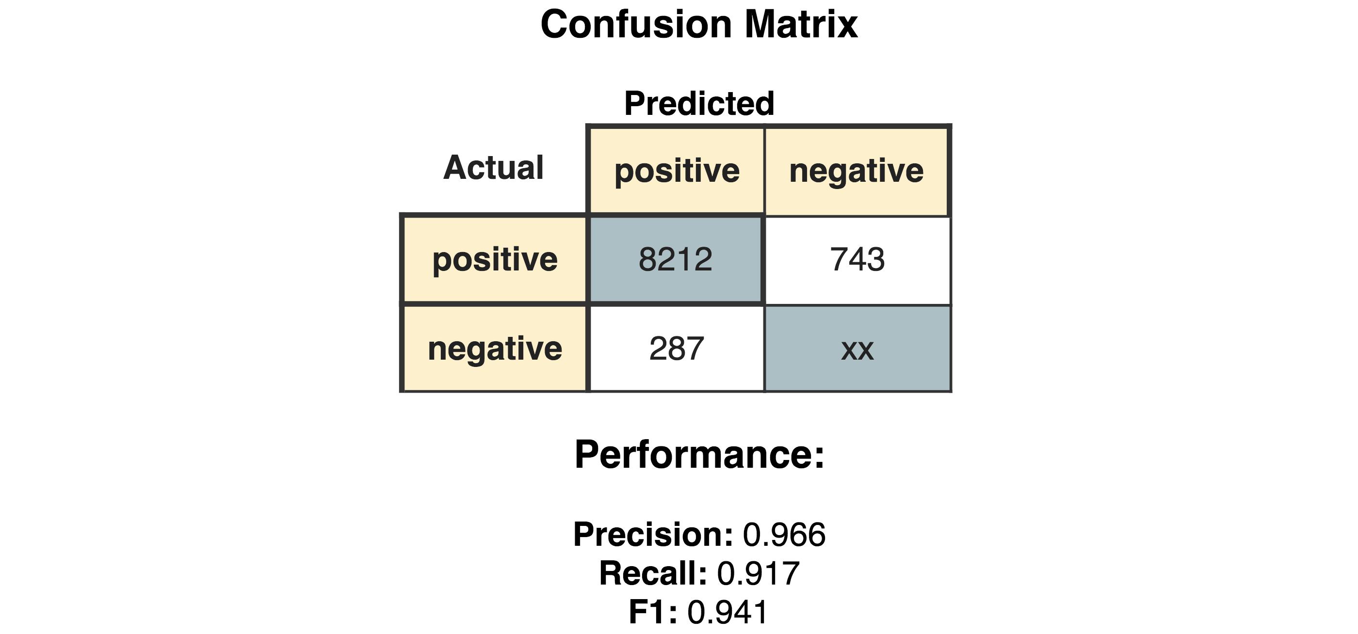
Next, we tag the documents in our test data with our trained model. Subsequently, we use the same test data to score our model. This is done with the node “StanfordNLP NE Scorer”, which calculates quality measures like precision, recall, and F1-measures and counts the amount of true positives, false negatives, and false positives. Note that it does not make sense to calculate true negatives, as this would be every word that is correctly not tagged as a disease. Internally, the “StanfordNLP NE Scorer” node tags the incoming test document set with a dictionary tagger using our initial disease dictionary. After that, the documents are tagged again via the input model, and then the node calculates the differences between the tags created by the dictionary tagger and the tags created by the input model.
The “Generic JavaScript View” node helps us to generate a view summarizing the results. As can be seen in Figure 3, we achieve a Precision of 0.966, Recall of 0.917, F1 of 0.941.
Comparison with input dictionary
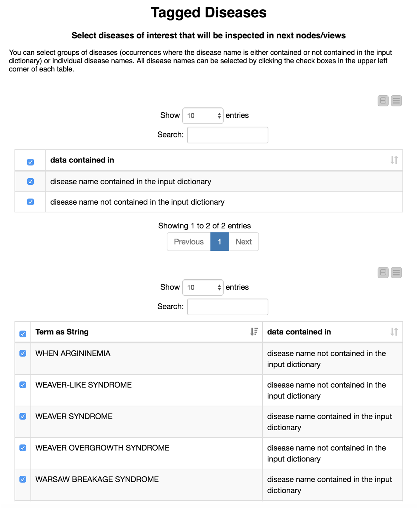
Now comes the interesting part. We are not only interested in how well our model recaptures disease names that we already know, but also if we are able to find new disease names. Therefore, we divide the diseases we have found in the test set depending on whether or not they were in our initial dictionary. We flag these either as “disease name contained in the input dictionary” or, alternatively, as “disease name NOT contained in the input dictionary.”
We then create an interactive view that allows the user to investigate and filter the results. This view is depicted in Figure 4. To select all data that were(or were not) contained in the input we use a “GroupBy” node to group according to the attribute we just created (i.e., if the data were part of the input dictionary or not). Here we use a small trick: it is important to “Enable highlighting” in the GroupBy node. If we show that in a composite view using a Table View (JavaScript) alongside another JavaScript view, it is now possible to make selections in one view which affect the other as well. If the user does not select anything, we will use all diseases by default.
This part is included in the metanode named “Compare with input dictionary”
The disease names detected in the test set that are not contained in the input dictionary can be very similar to the ones that we used for the training. For example, PYCNODYSOSTOSIS is contained in our input dictionary and we detect the new name PYCNODYSOSTOSIS SYNDROME as well as the misspelling PYCNODYSOTOSIS, which we flag as not part of the input dictionary. The similarity of the tags shows us that the tagged disease names that are not part of the input dictionary actually do make sense. These alternate tags can be valuable, for example, in normalization efforts where we need to determine synonyms and/or spelling variants of disease names.
To learn more about the newly detected disease names where the relationship to our input is less clear, we investigate whether or not tagged disease names co-occur in the same documents. This enables us to, for example, infer information from known diseases to the ones that were not in the input dictionary.
3. Co-occurence of Tagged Diesease Names
In this last part, we utilize the node “Term Co-Occurrence Counter” to count the number of co-occurrences for the list of tagged diseases within the documents. We add the information to the resulting disease pairs pertaining to whether or not each term was part of the input dictionary.
Co-occurrence network
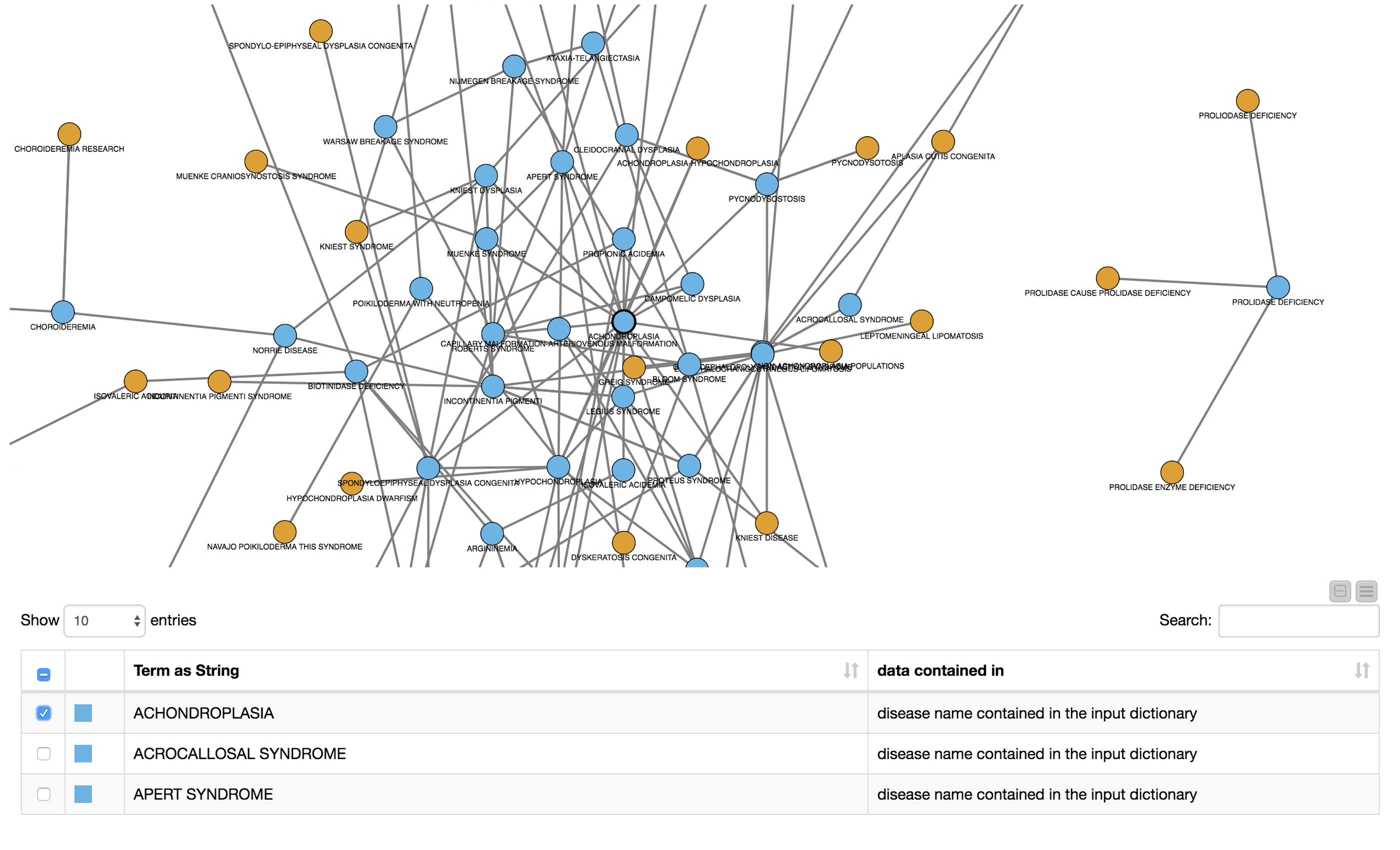
To facilitate the investigation of the results, we created a network graph with diseases as nodes, which were connected if they co-occurred in the same document. We colored the nodes according to their flag specifying whether or not they were contained in the input dictionary. We then created a view containing the network as well as a table with the disease names and the annotation stating whether it was part of the input dictionary. The creation of the network graph, node assignment, coloring, and edge definition is all computed in the metanode named “Co-oc Network”. The view is shown in Figure 5.
The user can now select nodes or rows of interest for further inspection either in the network or in the table. The subgraph surrounding the selected nodes/rows will be extracted and displayed in the next metanode.
Subgraph
The KNIME node “SubGraph Extractor” enables us to focus on a specific subset of diseases and their neighbors in the co-occurrence network. For that, the user needs to select a disease of interest. If nothing is selected we display a message stating that one did not select a disease to inspect in subgraph. We utilize the “Try” and “Catch Error” nodes to check if the selection is empty.

Again, we show the network (Network Viewer node) in an interactive view along with a table (Table View node) containing the disease names. Furthermore, we display additional information about genetic associations of the disease in the same table. We do this by joining the edge table of our network with genetic information about the diseases that we collected from Ensembl Biomart (see Fig. 6). This allows us to derive hypotheses about the genetic basis of the diseases that were not in our input dictionary.
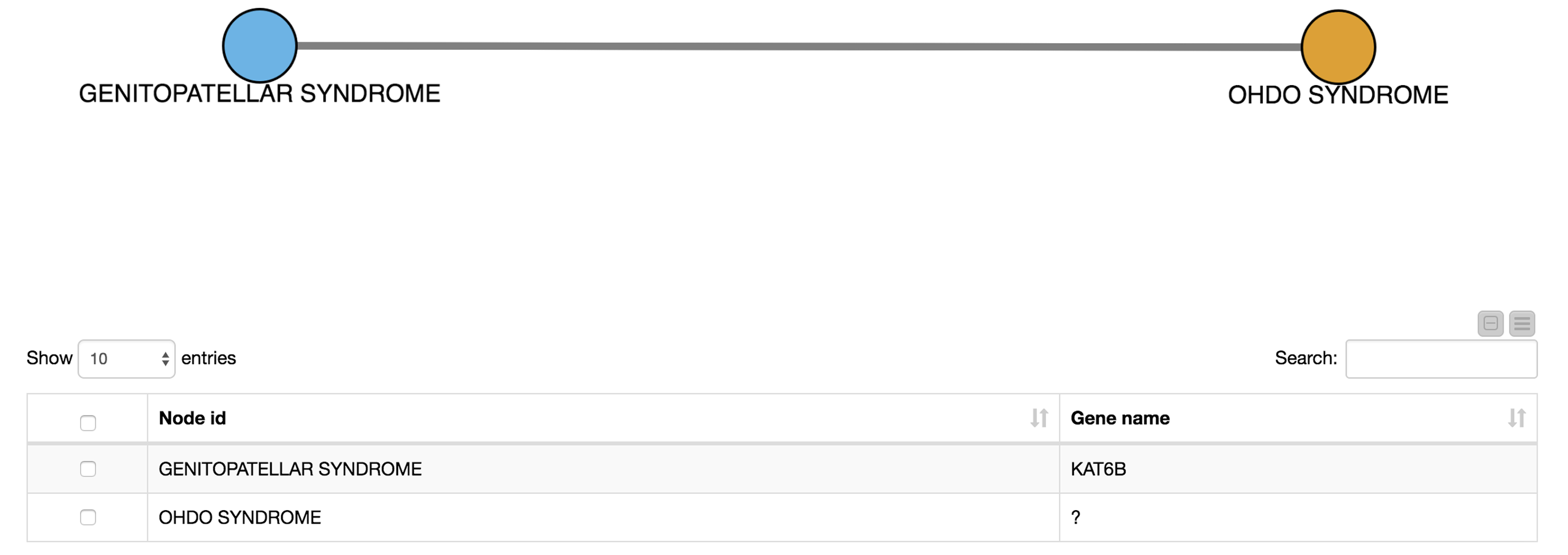
For example, we select OHDO SYNDROME, which was not part of our input dictionary. In the resulting view (Fig. 7), we see that this disease co-occurs with GENITOPATELLAR SYNDROME. Using the Ensembl information, we know that GENITOPATELLAR SYNDROME is associated with the gene, KAT6B. This could lead to the working hypothesis that OHDO SYNDROME is also associated with KAT6B. Indeed, mutations in the KAT6B gene have been associated with the Say-Barber-Biesecker Variant of Ohdo Syndrome3.
Summary
Today, we successfully trained a model to tag disease names in biomedical abstracts from PubMed. We started with a set of well known disease names in a dictionary. We then interactively investigated these known diseases as well as diseases that were not in our original dictionary and checked their co-occurrence in the collected documents. From these co-occurrences, we created a co-occurrence network where we could easily zoom into connected subgraphs and their underlying genetic associations.
In summary, we learned how to tag new and known disease names in KNIME Analytics Platform, and hopefully you had fun!
References
1 (2013, August 21). DNorm: disease name normalization with pairwise learning to rank. Retrieved July 12, 2018, from https://www.ncbi.nlm.nih.gov/pmc/articles/PMC3810844/
2 (2006, February 1). Literature mining for the biologist: from information retrieval to ... - Nature. Retrieved July 12, 2018, from https://www.nature.com/articles/nrg1768
3 "Whole-exome-sequencing identifies mutations in histone ... - NCBI." 11 Nov. 2011, https://www.ncbi.nlm.nih.gov/pubmed/22077973. Accessed 1 Aug. 2018.
