Learn 3 approaches to predict credit card fraud

According to the Nilson Report, global card fraud losses amounted to $21.84 billion in 2016, an increase of 4.4% over 2015. This confirms the importance of early detection of fraud in credit card transactions. With global credit card fraud loss on the rise, it is important for banks, as well as e-commerce companies, to be able to detect fraudulent transactions before they are completed. In this article we show you three approaches to predict credit card fraud using random forest, neural encoder, and isolation forest.

Fraud detection in credit card transactions is a very wide and complex field. Over the years, a number of techniques have been proposed, mostly stemming from the anomaly detection branch of data science. That said, most of these techniques can be reduced to two main scenarios depending on the available dataset:

1. Scenario 1: The dataset has a sufficient number of fraud examples.
2. Scenario 2: The dataset has no (or just a negligible number of) fraud examples.

In the first scenario, we can deal with the problem of fraud detection by using classic machine learning or statistics-based techniques. We can train a machine learning model or calculate some probabilities for the two classes (legitimate transactions and fraudulent transactions) and apply the model to new transactions so as to estimate their legitimacy. All supervised machine learning algorithms for classification problems work here, e.g., random forest, logistic regression, etc.

In the second scenario, we have no examples for fraudulent transactions, so we need to get a bit more creative. Since all we have are examples of legitimate transactions, we need to make them suffice. There are two options for that: We can treat fraud as an outlier or as an anomaly and use a consistent approach.

• Option one, a classic example for anomaly detection, is the neural autoencoder
• Option two, for the outlier detection approach, is the isolation forest algorithm.

Let’s take a look at how the different techniques can be used in practice on a real dataset. We implemented them on the fraud detection dataset from Kaggle. This dataset contains 284,807 credit card transactions, which were performed in September 2013 by European cardholders. Each transaction is represented by:

• 28 principal components extracted from the original data
• the time from the first transaction in the dataset
• the amount of money

The transactions have two labels: 1 for fraudulent and 0 for legitimate (normal) transactions. Only 492 (0.2%) transactions in the dataset are fraudulent, which is not really that many, but it may still be enough for some supervised training. Notice that the data contain principal components instead of the original transaction features, for privacy reasons.

Let’s start with the first scenario where we assume that a labeled dataset is available to train a supervised machine learning algorithm on a classification problem. Here we can follow the classical steps of a data science project: data preparation, model training, evaluation and optimization, and, finally, deployment.

Data preparation usually involves:

• Missing value imputation, if required then by the upcoming machine learning algorithm
• Feature selection for improved final performance
• Additional data transformations to comply with the most recent regulations on data privacy

However, in this case, the dataset we chose has already been cleaned, and it is ready to use; no additional data preparation is needed.

All supervised classification algorithms need a training set to train the model and a test set to evaluate the model quality. After reading, the data therefore have to be partitioned into a training set and a test set. Common partitioning proportions vary between 80-20% and 60-40%. For our example, we adopted 70-30% partitioning, where 70% of the original data is put into the training set, and the remaining 30% is reserved as the test set for the final model evaluation.

For classification problems like the one at hand, we need to ensure that both classes — in our case, fraudulent and legitimate transactions — are present in the training and test sets. Since one class is much less frequent than the other, stratified sampling is advised here rather than random sampling. Indeed, while random sampling might miss the samples from the least numerous class, stratified sampling guarantees that both classes are represented in the final subset according to the original class distribution.

Any supervised machine learning algorithm could work. For demonstration purposes, we have chosen a random forest with 100 trees, all trained up to a depth of ten levels and with a maximum of three samples per node, using the information gain ratio as a quality measure for the split criterion.

After the model has been trained, it has to be evaluated on the test set. Classic evaluation metrics can be used, such as sensitivity and specificity, or Cohen’s Kappa. All of these measures rely on the predictions provided by the model. In most data analytics tools, model predictions are produced based on the class with the highest probability, which in a binary classification problem is equivalent to using a default 0.5 threshold on one of the class probabilities.

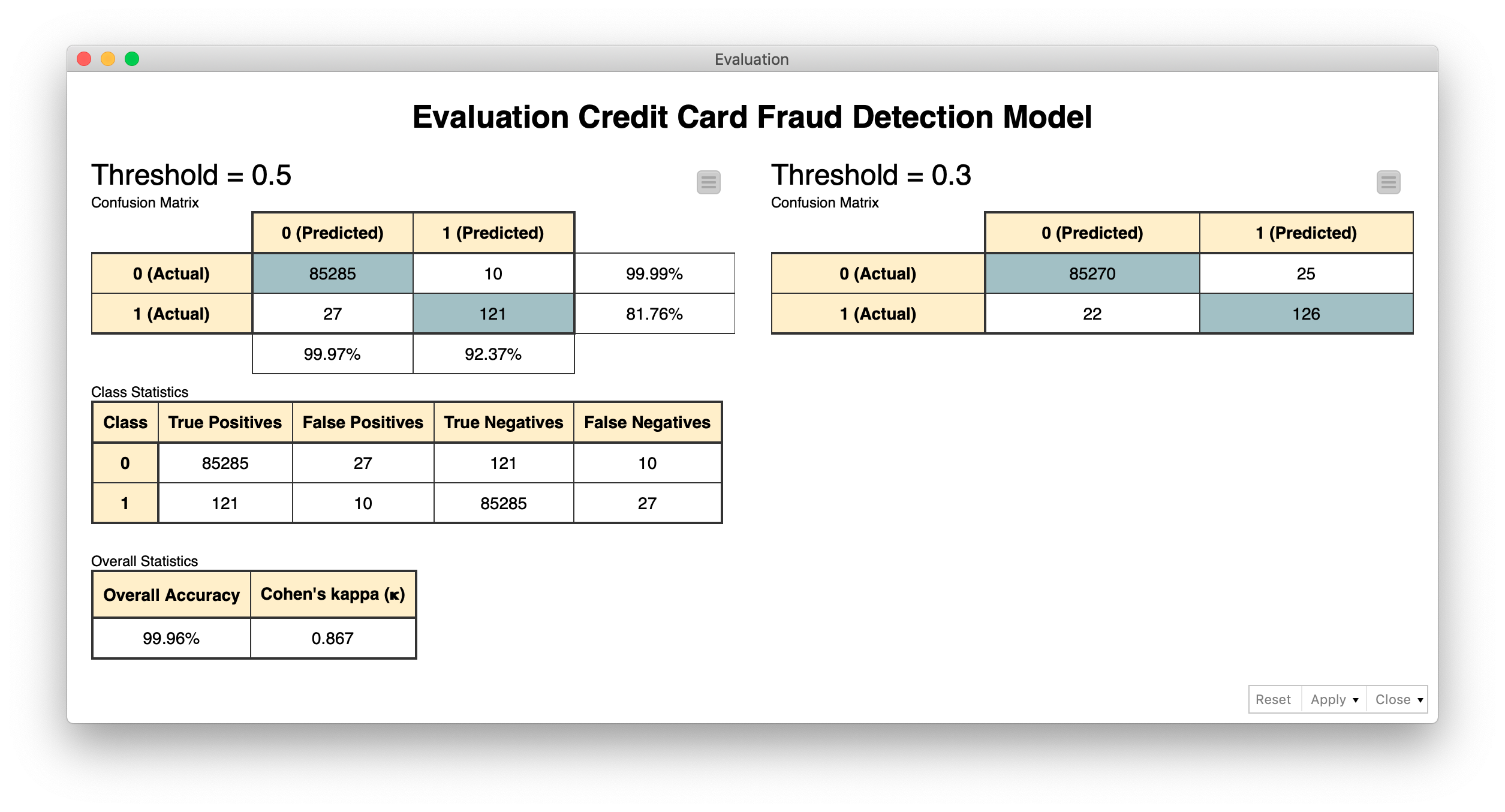
However, in the case of fraud detection, we might want to be more conservative regarding fraudulent transactions. This means we would rather double-check a legitimate transaction and risk bothering the customer with a potentially useless call rather than miss out on a fraudulent transaction. In this case, the threshold of acceptance for the fraudulent class is lowered — or alternatively, the threshold of acceptance for the legitimate class is increased. For this case study, we adopted a decision threshold of 0.3 on the probability of the fraudulent class and compared the results with what we obtained with the default threshold of 0.5.

In the figure below, you can see the confusion matrices obtained using a decision threshold of 0.5 (on the left) and 0.3 (on the right), leading respectively to Cohen’s Kappa of 0.890 and 0.898 on an undersampled dataset with the same number of legitimate and fraudulent transactions. As you can see from the confusion matrices, privileging the decision toward fraudulent transactions produces a few additional legitimate transactions mistaken as fraudulent as the price to pay for more fraudulent transactions correctly identified.

To complete the training cycle, the model parameters could be optimized — as for all classification solutions. We have omitted this part in this case study, but it could easily be introduced. For a random forest, this means finding the optimal number of trees and tree depth for the best classification performance (D. Goldmann, "Stuck in the Nine Circles of Hell? Try Parameter Optimization and a Cup of Tea," KNIME Blog, 2018; Hyperparameter optimization). In addition, the prediction threshold could also be optimized.

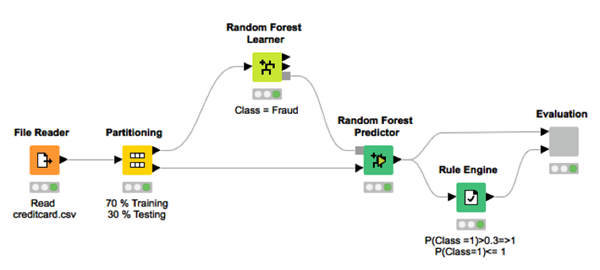
The workflow we used for training is therefore a very simple one with just a few nodes (Fig. 2): reading, partitioning, random forest training, random forest prediction generation, threshold application, and performance scoring.

• Download the workflow Fraud Detection: Model Training for free from the KNIME Hub.

Finally, when the model performance is acceptable by our standards, we can use it in production on real-world data.

The deployment workflow (Fig. 3) imports the trained model, reads one new transaction at a time, and applies the model to the input transaction and the custom threshold to the final prediction. In the event that a transaction is classified as fraudulent, an email is sent to the credit card owner to confirm the transaction’s legitimacy.

Let’s now move on to the second scenario. The fraudulent transactions in the dataset were so few anyway that they could simply be reserved for testing and completely omitted from the training phase.

One of the approaches that we have proposed stems from anomaly detection techniques. Anomaly detection techniques are often used to detect any exceptional or unexpected event in the data, be it a mechanical piece failure in IoT, an arrhythmic heartbeat in the ECG signal, or a fraudulent transaction in the credit card business. The complex part of anomaly detection is the absence of training examples for the anomaly class.

A frequently used anomaly detection technique is the neural autoencoder: a neural architecture that can be trained on only one class of events and used in deployment to warn us against unexpected new events. We will describe its implementation here as an example for the anomaly detection techniques.

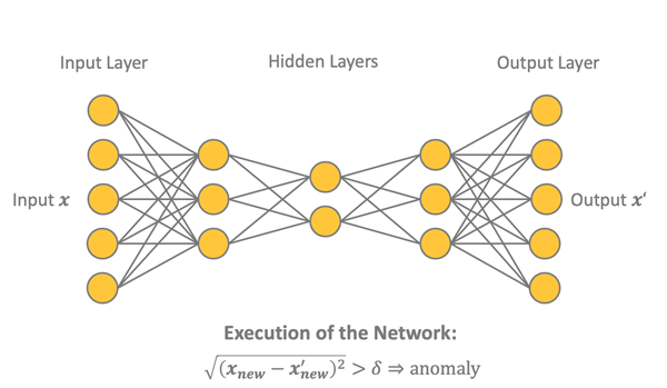
As shown below in figure 4, the autoencoder is a feed-forward backpropagation-trained neural network with as many n input units as n output units. In the middle, it has one or more hidden layers with a central bottleneck layer with h units.

The autoencoder is trained using only examples from one of the two classes, in this case the class of legitimate transactions. During deployment, the autoencoder will therefore perform a reasonable job in reproducing the input x on the output layer x' when presented with a legitimate transaction and a less than optimal job when presented with a fraudulent transaction (i.e., an anomaly). This difference between x and x' can be quantified via a distance measure, e.g.,

The final decision on legitimate transaction vs. fraudulent transaction is taken using a threshold value δ on the distance d(x,x'). A transaction x is a fraud candidate according to the following anomaly detection rule:

The threshold value δ can, of course, be set conservatively to fire an alarm only for the most obvious cases of fraud or can be set less conservatively to be more sensitive toward anything out of the ordinary. Let’s see the different phases involved in this process.

The first step in this case is to isolate a subset of legitimate transactions to create the training set in order to train the network. Of all legitimate transactions in the original dataset, 90% of them were used to train and evaluate the autoencoder network and the remaining 10%, together with the remaining fraudulent transactions, to build the test set for the evaluation of the whole strategy.

The usual data preparation steps should apply to the training set, as we discussed above. However, as we have also seen before, this dataset has already been cleaned, and it is ready to be used. No additional classic data preparation steps are necessary; the only step we need to take is a neural network custom required step: normalization of the input vectors to fall in [0,1].

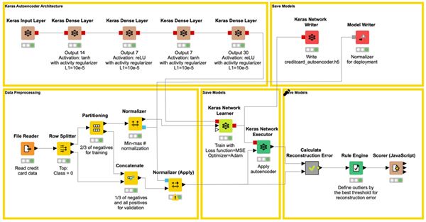
The autoencoder network is defined as a 30-14-7-7-30 architecture, using tanh and ReLU activation functions and activity regularizer L1 = 0.0001, as suggested in the blog post "Credit Card Fraud Detection using Autoencoders in Keras — TensorFlow for Hackers (Part VII)" by Venelin Valkov. The activity regularization parameter L1 is a sparsity constraint, which makes the network less likely to overfit the training data.

The network is trained until the final loss values are in the range [0.070, 0.071], according to the loss function mean squared error (MSE):

where N is the batch size and n is the number of units on the output and input layer.

The number of training epochs is set to 50, the batch size N is also set to 50, and Adam— an optimized version of the backpropagation algorithm — is chosen as the training algorithm. After training, the network is saved for deployment as a Keras file.

Model evaluation: making an informed decision

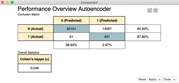
The value of the loss function, however, does not tell the whole story. It just tells us how well the network is able to reproduce "normal" input data onto the output layer. To get a full picture of how well this approach performs in detecting fraudulent transactions, we need to apply the anomaly detection rule mentioned above to the test data, including the few frauds.

In order to do this, we need to define the threshold δ for the fraud alert rule. A good starting point for the threshold comes from the final value of the loss function at the end of the learning phase. We used δ = 0.009, but as mentioned earlier, this is a parameter that could be adapted depending on how conservative we want our network to be.

The final workflow — building the autoencoder neural network, partitioning the data into training and test set, normalizing the data before feeding them into the network, training the network, applying the network to the test data, calculating the distance d(x,x'), applying the threshold δ, and finally scoring the results — is shown in figure 6.

Tip: Download the Keras Autoencoder for Fraud Detection Training workflow from the KNIME Hub.

We've now reached the deployment phase. In the deployment application, the trained autoencoder is read and applied to the new normalized incoming data, the distance between input vector and output vector is calculated, and the threshold is applied. If the distance is below the threshold, the incoming transaction is classified as legitimate, otherwise as fraudulent.

Notice that the network plus threshold strategy has been deployed within a REST application, accepting input data from the REST Request and producing the predictions in the REST Response.

The workflow implementing the deployment is shown in figure 7.

Tip: Download the Keras Autoencoder for Fraud Detection Deployment workflow from the KNIME Hub.

Another group of strategies for fraud detection — in the absence of enough fraud examples — relies on techniques for outlier detection. Among all of the many available outlier detection techniques, we propose the isolation forest technique (M. Widmann and M. Heine, "Four Techniques for Outlier Detection," KNIME Blog, 2019).

The basic idea of the isolation forest algorithm is that an outlier can be isolated with less random splits than a sample belonging to a regular class, as outliers are less frequent than regular observations and have values outside of the dataset statistics.

Following this idea, the isolation forest algorithm randomly selects a feature and randomly selects a value in the range of this feature as the split value. Using this partitioning step recursively generates a tree. The number of required random splits (the isolation number) to isolate a sample is the tree depth. The isolation number (often also called the mean length), averaged over a forest of such random trees, is a measure of normality and our decision function to identify outliers. Random partitioning produces noticeably shorter tree depths for outliers and longer tree depths for other data samples. Hence, when a forest of random trees collectively produces shorter path lengths for a particular data point, this is likely to be an outlier.

Again, the data preparation steps are the same as mentioned above: missing value imputation, feature selection, and additional data transformations to comply with the most recent regulations on data privacy. As this dataset has already been cleaned, it is ready to be used. No additional classic data preparation steps are necessary. The training and test sets are created in the same way as in the autoencoder example.

Thus, an isolation forest with 100 trees and a maximum tree depth of eight is trained, and the average isolation number for each transaction across the trees in the forest is calculated.

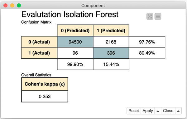
Remember, the average isolation number for outliers is smaller than for other data points. We adopted a decision threshold δ=6. Therefore, a transaction is defined as a fraud candidate if the average isolation number lies below that threshold. As in the other two examples, this threshold is a parameter that can be optimized, depending on how sensitive we want the model to be.

Performances for this approach on the test set are shown in Fig. 8.

Tip: Download the final Isolation Forest for Fraud Detection Training workflow, from the KNIME Hub.

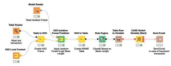
The deployment application here reads the isolation forest model and applies it to the new incoming data. Based on the threshold defined during training and applied to the isolation number value, the incoming data point is identified as either a candidate fraud transaction or a legitimate transaction.

1. Fraud detection techniques mostly stem from the anomaly detection branch of data science
2. If the dataset has a sufficient number of fraud examples, supervised machine learning algorithms for classification like random forest or logistic regression can be used for fraud detection
3. If the dataset has no fraud examples, we can use either the outlier detection approach using isolation forest technique or anomaly detection using the neural autoencoder
4. After the machine learning model has been trained, it's evaluated on the test set using metrics such as sensitivity and specificity, or Cohen’s Kappa

As described at the beginning of this tutorial, fraud detection is a wide area of investigation in the field of data science. We have portrayed two possible scenarios depending on the available dataset: a dataset with data points for both classes of legitimate and fraudulent transactions and a dataset with either no examples or only a negligible number of examples for the fraud class.

For the first scenario, we suggested a classic approach based on a supervised machine learning algorithm, following all the classic steps in a data science project as described in the CRISP-DM process. This is the recommended way to proceed. In this case study, we implemented an example based on a random forest classifier.

Sometimes, due to the nature of the problem, no example for the class of fraudulent transactions is available. In these cases, less accurate approaches which are nevertheless still feasible become appealing. For this second scenario, we have described two different approaches: the neural autoencoder from the anomaly detection techniques and the isolation forest from the outlier detection techniques. As in our example, often both of them are not as accurate as the random forest, but in some cases, we have no other possible approach to use.

The three approaches proposed here are surely not the only ones that can be found in literature. However, we believe that they are representative of the three commonly used groups of solutions for the fraud detection problem.

Notice that the last two approaches were discussed for cases in which labeled fraud transactions are not available. These are kind of emergency approaches, to be used when the classic approach for classification cannot be applied for lack of labeled data in the fraud class. We recommend using a supervised classification algorithm whenever possible. However, when no fraud data is available, one of the last two approaches could be of help. Indeed, while being prone to produce false positives, they are in some cases the only possible ways to deal with the problem of fraud detection.

As first published in InfoQ.