KNIME and Jupyter

KNIME user: You got your notebook in my workflow!

Jupyter Python user: You got your workflow in my notebook!

Both: Oooo, they work great together! ¹

KNIME Analytics Platform has had good integration with Python for quite a while. Since we think it’s important, we continue to invest in making improvements. Since the 3.7 release of KNIME Analytics Platform:

1. You can now use the Python code found in Jupyter notebooks from the Python scripting nodes in KNIME
2. You can now execute KNIME workflows directly from within Python. If you are working within a Jupyter notebook you can also get a (static) view of the workflow in the notebook.

We’ve made a couple of short videos demonstrating the new functionality. One on using Code from Jupyter in KNIME Analytics Platform and the other on using KNIME Workflows in Jupyter Notebooks. In this post we get into a bit more depth about what you can do.

Let’s start with using code from Jupyter notebooks from inside of KNIME.

I almost always end up using Jupyter when I’m trying out something new in Python. I really appreciate the way input and the resulting output are captured together, the matplotlib integration, and the ability to make notes about what I’m doing. For this blog post we’ll look at a concrete example of this.

At the end of last year I was exploring additional things we could learn from the documents that Jeany, here at KNIME, exported from PubChem as part of her Fun with Tags blog post. I built a topic model for the documents (for more information on that: Kilian, from our Berlin office, wrote a nice blog post about topic modeling) and wanted some way to visualize and explore the results.

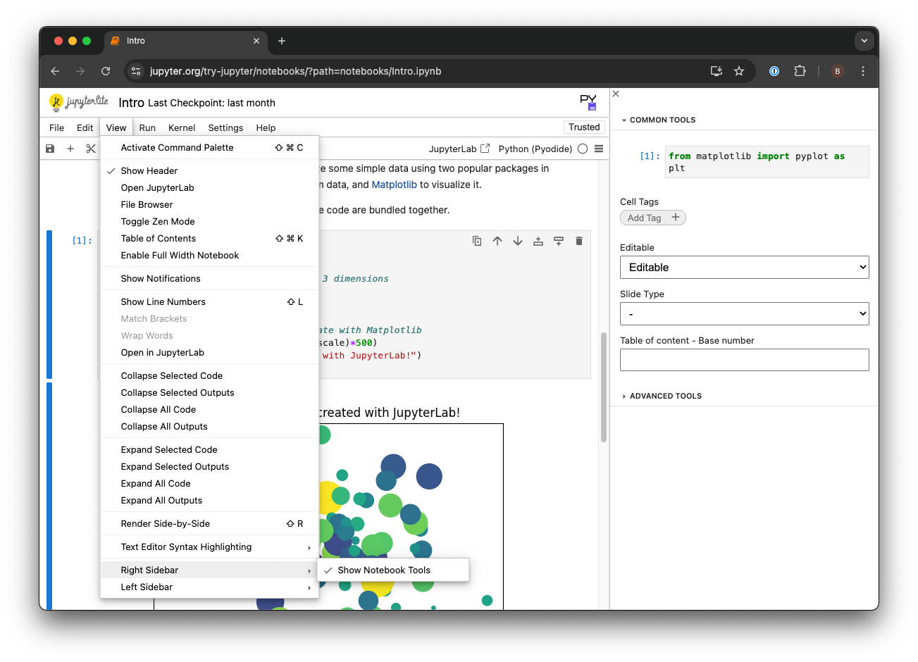
An obvious first step was to project the documents from the high-dimensional topic space into two dimensions and then just do a scatter plot. KNIME has nodes for doing this kind of thing (e.g. the PCA and MDS nodes), but I knew that I’d eventually want to do this on a large dataset, so I decided to give t-SNE (t-Distributed Stochastic Neighbor Embedding) a try. I hadn’t previously worked with t-SNE, so I put together a Jupyter notebook that I could use to try things out: https://gist.github.com/greglandrum/88d1739577c26b01e871d83c60c8898e. For the purposes of this blog post the most important part of the notebook is the cell defining a function for embedding data from a list of vectors (or numpy array), see Figure 1.

Once I had convinced myself that I could make the scikit-learn t-SNE code work, I was ready to move to KNIME and embed some documents.

Have a look at the workflow:

We start by:

• Reading in the ~10K saved documents

• Doing some preprocessing

• Building a topic model with 100 topics (I picked 100 arbitrarily here)

• Picking a subset of the documents by taking those retrieved by 10 random queries; in this case ~770 documents remain

The documents are then:

• Embedded using the Python scripting node (more on this in a moment)

• Finally the results are displayed using the “Interactive visualization” wrapped metanode

The view on this node has a scatter plot with a point for each document (colored by the query that retrieved the document) and two tables: the left table contains information about the selected documents and the right table contains information about the terms defining the topics to which the selected documents are assigned, as you can see in Figure 3.

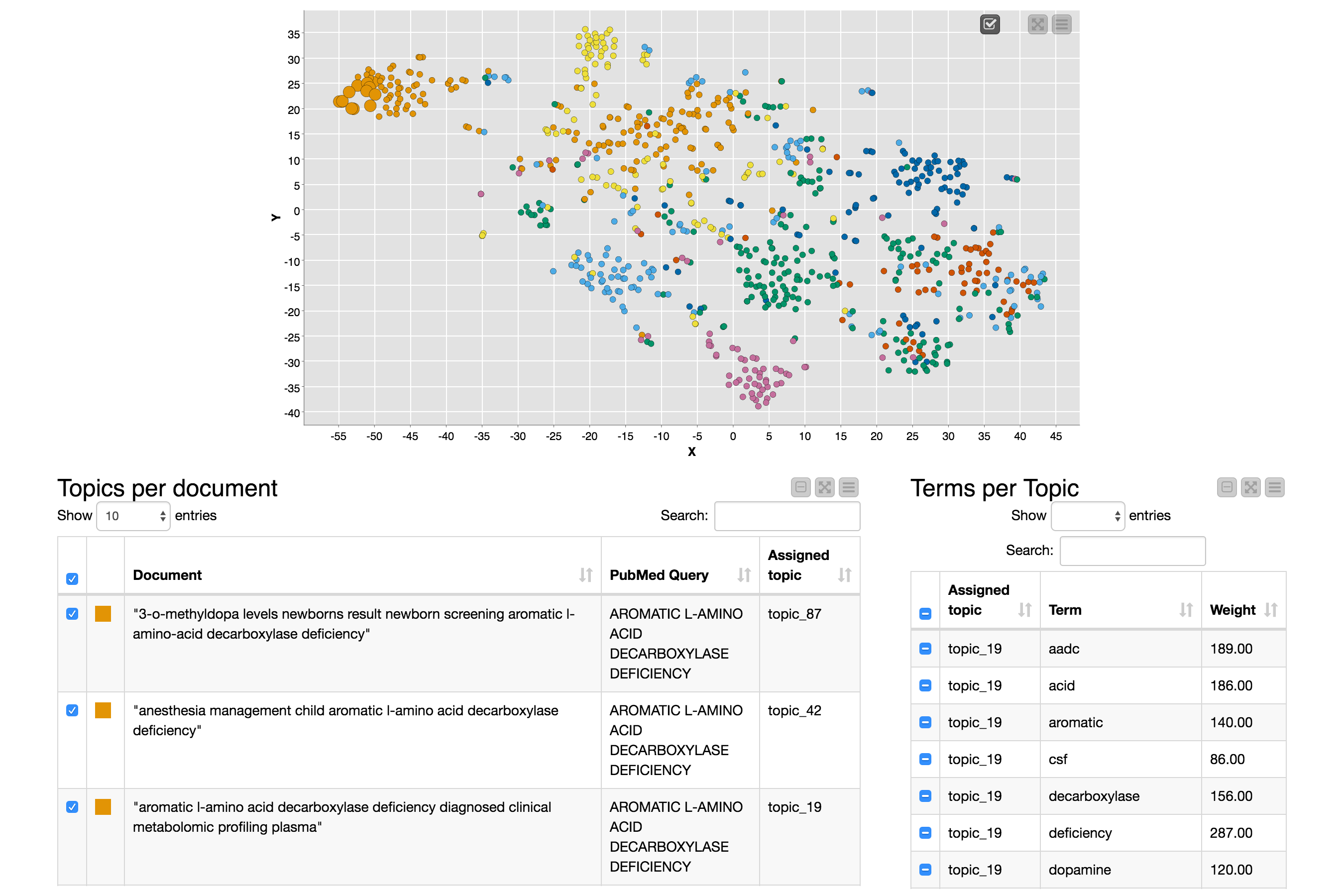
The view is cool and very useful for exploring the documents and the topics, and you should definitely try it out, but the main point of this blog post is the embedding process that produced the X and Y coordinates that are used in the scatter plot, so let’s come back to that.

In earlier versions of KNIME Analytics Platform I could have copied the Python code out of the Jupyter notebook cell shown in Figure 1, pasted it into the configuration dialog of a Python Script node, and everything would have been fine. This is perfectly functional, but becomes a coordination pain if I want to use the same code in multiple places and/or modify it. The new Jupyter integration added in KNIME 3.7 makes things a lot easier, see Figure 4.

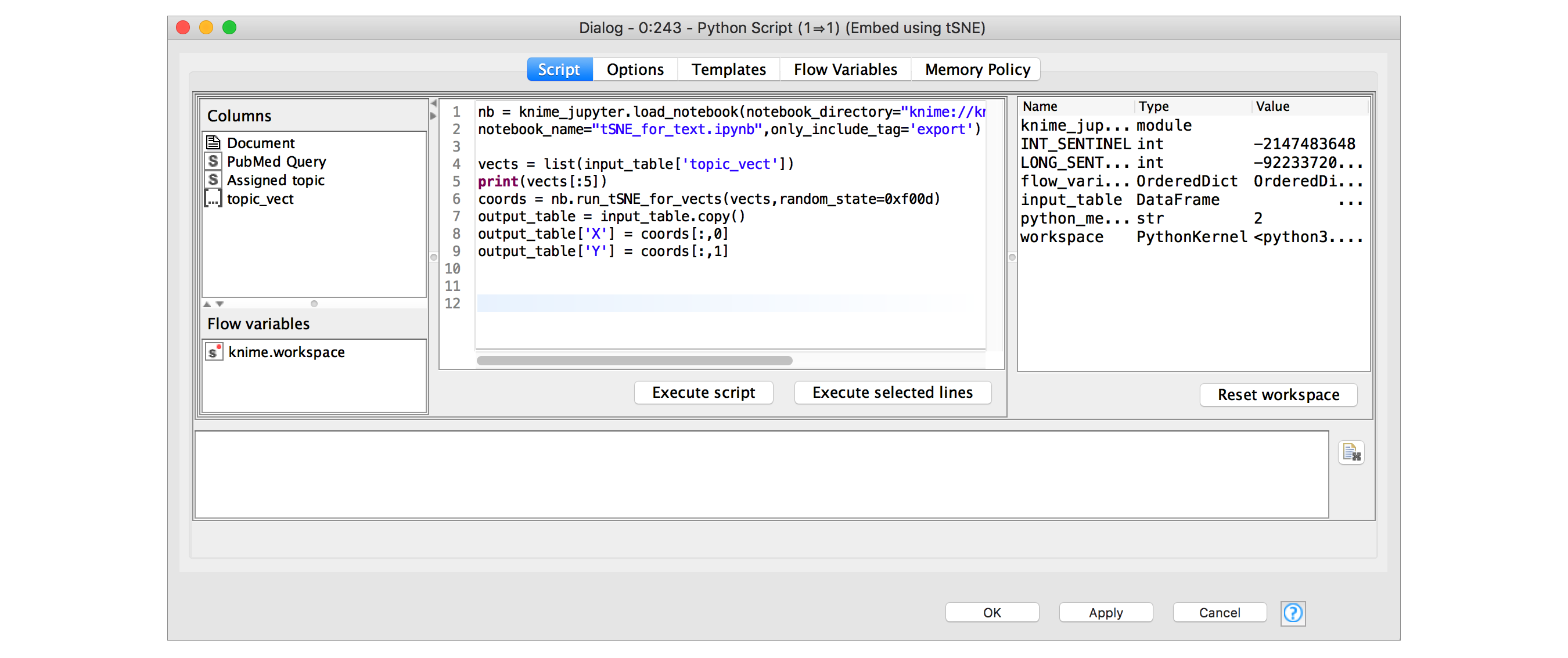
Using the knime_jupyter package, which is automatically available in all of the KNIME Python Script nodes, I can load the code that’s present in a notebook and then use it directly.

I do this as follows:

• Call load_notebook with the path to the directory containing my notebook and the name of the notebook. The notebook object that load_notebook returns provides access to all the functions and variables defined in the notebook itself²

• Use the run_tSNE_for_vects function, shown in Figure 1 above, to generate 2D coordinates for our documents

• Finally, add the results from the embedding as two new columns to the output table

Using the knime_jupyter package, which is automatically available in all of the KNIME Python Script nodes, I can load the code that’s present in a notebook and then use it directly.

Another useful feature is that you can easily call KNIME workflows from within a Jupyter notebook (or from other Python scripts).

In order to do this you need to first install the knime python package from PyPI by doing

. Once you have this package installed you’re ready to work with KNIME workflows in Python.

For this blog post we will be working with a workflow I built to query the ChEMBL database for information it has about biological targets and the bioactivities that have been measured for them, see Figure 5. The details of the query are encapsulated with the database connection information in the “Retrieve assays, activities, and targets” wrapped metanode. The rest of the workflow does a couple of different GroupBys on the results of that query and then filters them using a set of target IDs in a user-provided table (the “Container Input (Table)” node). The two different filtered tables are output using the “Container Output (Table)” nodes.

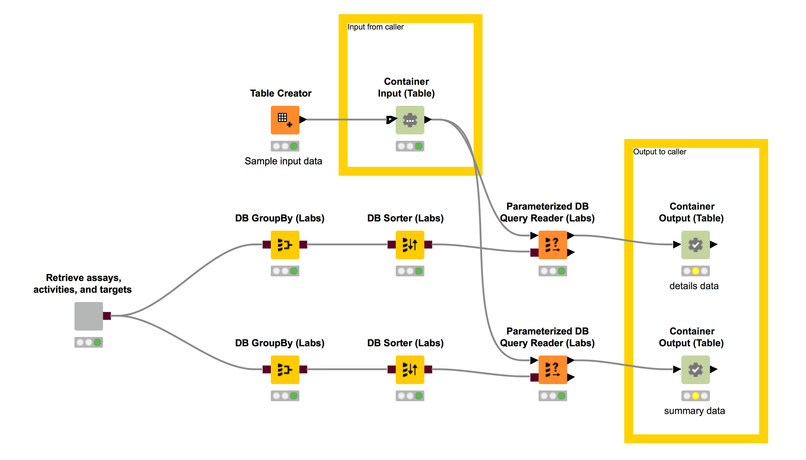
This workflow performs a type of query that I do fairly regularly and although it’s definitely possible to do this from Python (or directly within the Jupyter notebook using Catherine Devlin’s excellent %sql magic), I find it much easier to build and test complex database queries in KNIME.

Let’s see how to use this workflow from within Jupyter. The notebook I’m using is available here: https://gist.github.com/greglandrum/d721822e8973ff8438cf2af283c9271e. I start by importing the knime module in Python and telling it where my KNIME executable is (this isn’t necessary if KNIME is installed in a standard location):

Now I can open a KNIME workflow in Jupyter by providing the filesystem path to a KNIME workspace and the location of my workflow within that workspace (Figure 7).

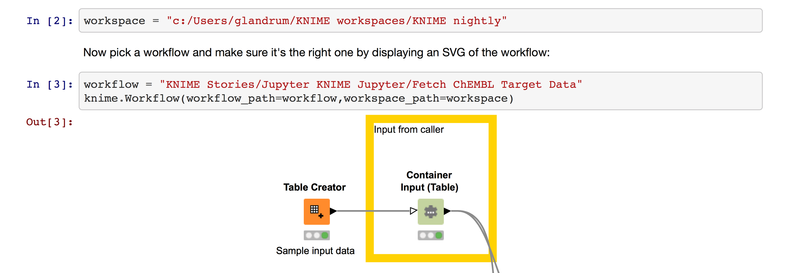
I’ve cut off the nice preview of the workflow in this screenshot, but you can see the full preview in the notebook itself.

I call the workflow by creating a Pandas DataFrame with the query table - in this case just containing a single column, setting that as the input for the workflow, and then executing the workflow (Figure 8).

This launches KNIME Analytics Platform in the background, runs the workflow, and then returns control to Jupyter. I can now get the output tables from the workflow object (Figure 9).

The data are in Pandas DataFrames (Figure 10).

That’s it! I can now continue working with that data in Jupyter.

Note that though this demo uses the Jupyter notebook, the knime-py module can be used from standard Python as well.

In this blog post I’ve demonstrated some of the new Python functionality added to KNIME Analytics Platform v3.7. I showed how you can use code from Jupyter notebooks directly in your KNIME workflows and how you can call KNIME workflows from within Jupyter notebooks (or standard Python).

The KNIME workflows and Jupyter notebooks used in the blog post are all available on the KNIME Public EXAMPLES space:

• KNIME from Jupyter workflow: find it on the KNIME Hub here.

• Jupyter from KNIME workflow: find it on the KNIME Hub here.

^1. “Mmmm ‘KNIME’! Mmmm ‘Jupyter’! Delicious!” Anyone remember this ad?

^2. By default load_notebook works by importing the Python code that’s present in all of the code cells in the notebook. Because my example notebook includes examples and testing code, I only want KNIME to load some of the cells, so in the example shown in Figure 4, I told load_notebook to only import code from notebook cells that have been tagged “export”. Tagging things in the notebook is easy, just turn on display of tags from the View->Cell Toolbar menu.